Introduction
This course/book is designed as your 'second course' in programming. It is assumed you've done a first course which taught you the basics of programming in an interpreted language (probably either python or R), and have now had some experience at using these in your research.
You might have felt that your code is holding you back, and that if you could make it faster or use less memory you could take your analysis further. Or you might have got a solution but are unsure whether it's the right approach, or whether you could make it better.
Sometimes seeing the impressive (but sometimes intractable!) code and methods we use for research in bioinformatics can feel intimidating, and I feel there isn't much formal guidance on how to engineer your code this way.
My hope is that this course will give you some extra skills and confidence when developing and improving your research code.
Content
- Optimising python code. We'll start with some ways to make your interpreted code faster, such as arrays, JIT compilation and sparse matrices.
- HPC. How to effectively use and monitor your computation on HPC systems, including compiling code with different options.
- Compiled languages. How using a statically typed language can be faster, how to control memory, and other pros/and cons (using rust as an example). Also understanding how your problem scales, and typical elements of your algorithmic toolbox to solve problems.
- Software engineering. How to turn your research code into a fully fledged software package.
- Recursion and closures. Some new patterns, with more challenging examples to implement.
- Parallel programming. Theory and examples for using multiple CPUs to parallelise code. Examples in multiple languages.
Possible future content
Future modules to be added (possibly):
- CUDA programming for GPU parallelism.
- Foreign function interfaces - linking your compiled code with R and python.
- Machine learning/deep learning.
- Cloud computing.
- Web development.
Resources
Some of this material is based on:
- 'Algorithms for Modern Hardware'. This goes into lots of detail, including a lot of assembly code. This would be good to read after this course, or if you want more evidence and theory behind optimisation.
- The rust book.
- C++ reference guide.
- Rust by practice
Prerequisites
Prerequisites
Before attending, you should be comfortable writing some code in python or R, including basics:
- Conditionals/if statements.
- Iteration.
- Reading from files, writing to files.
- Taking arguments on the command line.
- Use of functions.
- Data types.
- Data frames/arrays (R) or numpy arrays (python). Indexing into them.
It would also be helpful if you were familiar with:
- Plotting in ggplot2 or matplotlib.
- Some experience/use of functional programming, such as
lapplyin R.
Setup
- If you have a Windows computer, please install Ubuntu through WSL
- If you have a Mac, and it has an M1 chip, that you either have access to codon or you have set up conda with intel packages
- Install vscode, and extensions for python.
Session 2
- Make sure you have an account and can submit jobs on codon (at EBI) or a similar HPC environment at your own institution.
Session 3
- Install the rust toolchain, and check you can compile and run the test program.
- Install the rust-analyzer vscode extension. See the guide here https://code.visualstudio.com/docs/languages/rust.
- Check that you can debug a rust test program in vscode.
Session 4
- Set up a github account. You can get a pro account for free with an EBI email.
- Set up ssh key access for your github account.
Optimising python code
Some guiding principles:
- Only optimise code if you need to. By optimising it, will it be able to run on something you couldn't analyse otherwise? Will it save you more computation than the time it takes to optimise? Will lots of other people use the code, and therefore collectively save time?
- In my experience, going after >10x speedups is usually worth it as it hits the first two objectives. Going after ~2x speedups can often be worth it for commonly used programs, or that you intend to distribute as software. A 10% speedup is rarely worth it for research code -- this would be useful in library code used by thousands of people.
- Get the code to work before optimising it. It's helpful to have a test to ensure any changes you make haven't broken anything.
- Do your optimisation empirically, i.e. use a profiler. We're pretty bad at working out by intuition where the slow parts of the code are.
For now, we'll focus on a python example, but the ideas are similar in R.
- Counting codons
- Profiling
- Optimisation strategies
- Memory optimisation
- Writing extensions in compiled code
- Other optimisations
- Notes (for next year)
Counting codons
The first example we will work through is counting codons from a multiple sequence alignment.
A multiple sequence alignment stored in FASTA format might look something like:
>ERR016988;0_0_13
atgaaaaacactatgtctcctaaaaaaatacccatttggcttaccggcctcatcctactg
attgccctaccgcttaccctgccttttttatatgtcgctatgcgttcgtggcaggtcggc
atcaaccgcgccgtcgaactgttgttccgcccgcgtatgtgggatttgctctccaacacc
ttgacgatgatggcgggcgttaccctgatttccattgttttgggcattgcctgctccctt
ttgttccaacgttaccgcttcttcggcaaaaccttttttcagacggcaatcaccctgcct
ttgtgcatccccgcatttgtcagctgtttcacctggatcagcctgaccttccgtgtcgaa
ggcttttgggggacagtgatgattatgagcctgtcctcgttcccgctcgcctacctgccc
gtcgaggcggcactcaaacgcatcagcctgtcttacgaagaagtcagcctgtccttgggc
aaaagccgcctgcaaacctttttttccgccatcctcccccagctcaaacccgccatcggc
agcagcgtgttactgattgccctgcatatgctggtcgaatttggcgcggtatccattttg
aactaccccacttttaccaccgccattttccaagaatacgaaatgtcctacaacaacaat
accgccgccctgctttccgctgttttaatggcggtgtgcggcatcgtcgtatttggagaa
agcatatttcgcggcaaagccaagatttaccacagcggcaaaggcgttgcccgtccttat
cccgtcaaaaccctcaaactgcccggtcagattggcgcgattgtttttttaagcagcttg
ttgactttgggcattattatcccctttggcgtattgatacattggatgatggtcggcact
tccggcacattcgcgctcgtatccgtatttgatgcctttatccgttccttaagcgtatcg
gctttaggtgcgattttgactatattatgtgccttgccccttgtttgggcatcggttcgc
tatcgcaattttttaaccgtttggatagacaggctgccgtttttactgcacgccgtcccc
ggtttggttatcgccctatccttggtttatttcagcatcaactacacccctgccgtttac
caaacctttatcgtcgtcatccttgcctatttcatgctttacctgccgatggcgcaaacc
accctgaggacttccttggaacaactccccaaagggatggaacaggtcggcgcaacattg
gggcgcggacacttctttattttcaggacgttggtactgccgtccatcctgcccggcatt
accgccgcattcgcactcgtcttcctcaaactgatgaaagagctgaccgccaccctgctg
ctgaccaccgacgatgtccacacactctccaccgccgtttgggaatacacatcggacgca
caatacgccgccgccaccccttacgcgctgatgctggtattattttccggcatccccgta
ttcctgctgaagaaatacgccttcaaataa------------------------
>ERR016989;1_112_17
atgaaaaacactatgtctcctaaaaaaatacccatttggcttaccggcctcatcctactg
attgccctaccgcttaccctgccttttttatatgtcgctatgcgttcgtggcaggtcggc
atcaaccgcgccgtcgaactgttgttccgcccgcgtatgtgggatttgctctccaacacc
ttgacgatgatggcgggcgttaccctgatttccattgttttgggcattgcctgcgccctt
ttgttccaacgttaccgcttcttcggcaaaaccttttttcagacggcaatcaccctgcct
ttgtgcatccccgcatttgtcagctgtttcacctggatcagcctgaccttccgtgtcgaa
ggcttttgggggacagtgatgattatgagcctgtcctcgttcccgctcgcctacctgccc
gtcgaggcggcactcaaacgcatcagcctgtcttacgaagaagtcagcctgtccttgggc
aaaagccgcctgcaaacctttttttccgccatcctcccccagctcaaacccgccatcggc
agcagcgtgttactgattgccctgcatatgctggtcgaatttggcgcggtatccattttg
aactaccccacttttaccaccgccattttccaagaatacgaaatgtcctacaacaacaat
accgccgccctgctttccgctgttttaatggcggtgtgcggcatcgtcgtatttggagaa
agcatatttcgcggcaaagccaagatttaccacagcggcaaaggcgttgcccgtccttat
cccgtcaaaaccctcaacctccccggtcagattggcgcgattgtttttttaagcagcttg
ttgactttgggcattattatcccctttggcgtattgatacattggatgatggtcggcact
tccggcacattcgcgctcgtatccgtatttgatgcctttatccgttccttaagcgtatcg
gctttaggtgcggttttgactatattatgtgccttgccccttgtttgggcatcggtccgc
tatcgcaattttttaaccgtttggatagacaggctgccgtttttactgcacgccgtcccc
ggtttggttatcgccctatccttggtttatttcagcatcaactacacccctgccgtttac
caaacctttatcgtcgtcatccttgcctatttcatgctttacctgccgatggcgcaaacc
accctaaggacttccttggaacaactcccaaaagggatggaacaggtcggcgcaacattg
gggcgcggacacttctttattttcaggacgttggtactgccgtccatcctgcccggcatt
accgccgcattcgcactcgtcttcctcaaactgatgaaagagctgaccgccaccctgctg
ctgaccaccgacgatgtccacacactctccaccgccgtttgggaatacacatcggacgca
caatacgccgccgccaccccttacgcgctgatgctggtattattttccggcatccccgta
ttcctgctgaagaaatacgctttcaaataa------------------------
This format has sample headers which start > followed by the sample name, followed
by the sequence, wrapped at 80 characters to make it more human readable. Gaps are given by - characters.
We wish to count, at each aligned position, the number of observed codons for each of the 61 possible triplet positions plus the three stop codons TAG, TAA and TGA.
We'll use an example with aligned porB sequences from the bacterial pathogen Neisseria meningitidis, which you can download here.
Exercise Let's start off by writing some code in to read this file in and doing a simple check that the length is as expected (all the same, and a multiple of three). Let's also add some timing in, to see if we are improving when we add optimisations.
Have a go at this yourself, and then compare with the example below.
Example: read file
import time
import gzip

# Generator which keeps state after yield is called
# Based on a nice example: https://stackoverflow.com/a/7655072
def read_fasta_sample(fp):
    name, seq = None, []
    for line in fp:
        line = line.rstrip()
        if line.startswith(">"):
            if name: yield (name, ''.join(seq).upper())
            name, seq = line[1:], []
        else:
            seq.append(line)
    if name: yield (name, ''.join(seq).upper())

def read_file(file_name):
    n_samples = 0
    # Open either gzipped or plain file by looking for magic number
    # https://stackoverflow.com/a/47080739
    with open(file_name, 'rb') as test_f:
        zipped = test_f.read(2) == b'\x1f\x8b'
    if zipped:
        fh = gzip.open(file_name, 'rt')
    else:
        fh = open(file_name, 'rt')
    with fh as fasta:
        seqs = list()
        names = list()
        for h, s in read_fasta_sample(fasta):
            if len(s) % 3 != 0:
                raise RuntimeError(f"Sequence {h} is not a multiple of three")
            elif len(seqs) > 0 and len(s) != len(seqs[0]):
                raise RuntimeError(f"Sequence {h} is length {len(s)}, expecting {len(seqs[0])}")
            else:
                seqs.append(s)
                names.append(h)

    return seqs, names

def main():
    start_t = time.time_ns()
    seqs, names = read_file("BIGSdb_024538_1190028856_31182.dna.aln.gz")
    end_t = time.time_ns()
    time_ms = (end_t - start_t) / 1000000
    print(f"Time to read {len(seqs)} samples: {time_ms}ms")

if __name__ == "__main__":
    main()
Don't worry about perfecting your code at this point! Let's aim for something that runs easily and works, which we can then improve if we end up using it.
In the example above I have added a timer so we can try and keep track of how long
each section takes to run. A better way to do this would be to average over multiple
runs, for example using the timeit module, but some measurement is better than no
measurement.
I've made sure all the bases are uppercase so we don't have to deal with both
a and A in our counter, but I haven't checked for incorrect bases.
When I run this code, I see the following:
python example1.py
Time to read 4889 samples: 59.502ms
If I decompress the file first:
python example1.py
Time to read 4889 samples: 33.419ms
If you have a hard disk drive rather than a solid state drive, it is often faster to read compressed data and decompress it on the fly, as the speed of data transfer is the rate limiting step.
Exercise Now, using the sequences, write some code to actually count the codons. The output
should be a frequency vector at every site for every codon which does not
contain a -. Do this however you like.
Example: count codons
def count_codons(seqs):
    bases = ['A', 'C', 'G', 'T']
    codon_len = int(len(seqs[0]) // 3)
    counts = [dict()] * codon_len
    for seq in seqs:
        for codon_idx in range(codon_len):
            nuc_idx = codon_idx * 3
            codon = seq[nuc_idx:(nuc_idx + 3)]
            if all([base in bases for base in codon]):
                if codon in counts[codon_idx]:
                    counts[codon_idx][codon] += 1
                else:
                    counts[codon_idx][codon] = 1

    count_vec = list()
    for pos in counts:
        pos_vec = list()
        for base1 in bases:
            for base2 in bases:
                for base3 in bases:
                    codon = ''.join(base1 + base2 + base3)
                    if codon in pos:
                        pos_vec.append(pos[codon])
                    else:
                        pos_vec.append(0)

    return count_vec
Aside: debugging
My first attempt (above) was wrong and was returning an empty list. One way to look into this is by using a debugger.
Modern IDEs such as vscode and pycharm also let you run the debugger interactively, which is typically nicer than via the command line. However old school debugging is handy when you have to run your code on HPC systems, or with more complex projects such as when you have C++ and python code interacting.
python has pdb built-in, you can run it as follows:
python -m pdb example1.py
(gdb and lldb are equivalent debuggers for compiled code.)
Run help to see the commands. Most useful are setting breakpoints with b;
continuing execution with c, r, s and n; printing variables with p.
By stopping my code on the line with codon = ''.join(base1 + base2 + base3)
by typing b 62 to add a breakpoint, then r to run the code, I
can have a look at some counts:
p pos
{'ATG': 15401, 'TGA': 47348, 'GAA': 39489, 'AAA': 85118, 'AAT': 30105, 'ATC': 36135, 'TCC': 24440, 'CCC': 22958, 'CCT': 36610, 'CTG': 41756, 'GAT': 10002, 'ATT': 20458, 'TTG': 49731, 'TGC': 21500, 'GCC': 40734, 'GAC': 20218, 'ACT': 19778, 'CTT': 28321, 'TTT': 20797, 'TGG': 29906, 'GGC': 67370, 'GCA': 45599, 'CAG': 23779, 'AGC': 34794, 'TTC': 29469, 'TGT': 9964, 'GTT': 39620, 'CAA': 42858, 'GCT': 30373, 'ACG': 15084, 'CGT': 23916, 'TTA': 9198, 'TAC': 21812, 'ACC': 30370, 'GTA': 33903, 'CGG': 62505, 'CAC': 11408, 'CCA': 20119, 'CAT': 22822, 'TCA': 20719, 'AAG': 42061, 'CCG': 35604, 'GCG': 24592, 'TAG': 10002, 'AGA': 17961, 'AAC': 28534, 'CGC': 21035, 'CTC': 19077, 'TCT': 13737, 'GAG': 4230, 'ACA': 15865, 'GGA': 5578, 'GGT': 42665, 'GTC': 11842, 'AGG': 21378, 'GTG': 1830, 'TCG': 37628, 'GGG': 13214, 'TAA': 18253, 'CTA': 9810, 'TAT': 6398, 'ATA': 2220, 'CGA': 5452, 'AGT': 5939}
For starters, these seem far too high, as we wouldn't expect counts over the number of samples (4889).
Stopping at codon = seq[codon_idx:(codon_idx + 3)] I see:
(Pdb) p codon
'ATG'
This looks ok. I'll step through some of the next lines with n:
if codon in counts[codon_idx]:
(Pdb) p counts
[{}, {}, {}, {}, {}, {}, {}, {}, {}, {}, {}, {}, {}, {}, {}, {}, {}, {}, {}, {}, {}, {}, {}, {}, {}, {}, {}, {}, {}, {}, {}, {}, {}, {}, {}, {}, {}, {}, {}, {}, {}, {}, {}, {}
, {}, {}, {}, {}, {}, {}, {}, {}, {}, {}, {}, {}, {}, {}, {}, {}, {}, {}, {}, {}, {}, {}, {}, {}, {}, {}, {}, {}, {}, {}, {}, {}, {}, {}, {}, {}, {}, {}, {}, {}, {}, {}, {}, {
}, {}, {}, {}, {}, {}, {}, {}, {}, {}, {}, {}, {}, {}, {}, {}, {}, {}, {}, {}, {}, {}, {}, {}, {}, {}, {}, {}, {}, {}, {}, {}, {}, {}, {}, {}, {}, {}, {}, {}, {}, {}, {}, {},
{}, {}, {}, {}, {}, {}, {}, {}, {}, {}, {}, {}, {}, {}, {}, {}, {}, {}, {}, {}, {}, {}, {}, {}, {}, {}, {}, {}, {}, {}, {}, {}, {}, {}, {}, {}, {}, {}, {}, {}, {}, {}, {}, {},
 {}, {}, {}, {}, {}, {}, {}, {}, {}, {}, {}, {}, {}, {}, {}, {}, {}, {}, {}, {}, {}, {}, {}, {}, {}, {}, {}, {}, {}, {}, {}, {}, {}, {}, {}, {}, {}, {}, {}, {}, {}, {}, {}, {}
, {}, {}, {}, {}, {}, {}, {}, {}, {}]
Initialisation looks ok
> example1.py(51)count_codons()
-> counts[codon_idx][codon] = 1
(Pdb) n
> example1.py(45)count_codons()
-> for codon_idx in range(codon_len):
(Pdb) p counts
[{'ATG': 1}, {'ATG': 1}, {'ATG': 1}, {'ATG': 1}, {'ATG': 1}, {'ATG': 1}, {'ATG': 1}, {'ATG': 1}, {'ATG': 1}, {'ATG': 1}, {'ATG': 1}, {'ATG': 1}, {'ATG': 1}, {'ATG': 1}, {'ATG'
: 1}, {'ATG': 1}, {'ATG': 1}, {'ATG': 1}, {'ATG': 1}, {'ATG': 1}, {'ATG': 1}, {'ATG': 1}, {'ATG': 1}, {'ATG': 1}, {'ATG': 1}, {'ATG': 1}, {'ATG': 1}, {'ATG': 1}, {'ATG': 1}, {
'ATG': 1}, {'ATG': 1}, {'ATG': 1}, {'ATG': 1}, {'ATG': 1}, {'ATG': 1}, {'ATG': 1}, {'ATG': 1}, {'ATG': 1}, {'ATG': 1}, {'ATG': 1}, {'ATG': 1}, {'ATG': 1}, {'ATG': 1}, {'ATG':
1}, {'ATG': 1}, {'ATG': 1}, {'ATG': 1}, {'ATG': 1}, {'ATG': 1}, {'ATG': 1}, {'ATG': 1}, {'ATG': 1}, {'ATG': 1}, {'ATG': 1}, {'ATG': 1}, {'ATG': 1}, {'ATG': 1}, {'ATG': 1}, {'A
TG': 1}, {'ATG': 1}, {'ATG': 1}, {'ATG': 1}, {'ATG': 1}, {'ATG': 1}, {'ATG': 1}, {'ATG': 1}, {'ATG': 1}, {'ATG': 1}, {'ATG': 1}, {'ATG': 1}, {'ATG': 1}, {'ATG': 1}, {'ATG': 1}
, {'ATG': 1}, {'ATG': 1}, {'ATG': 1}, {'ATG': 1}, {'ATG': 1}, {'ATG': 1}, {'ATG': 1}, {'ATG': 1}, {'ATG': 1}, {'ATG': 1}, {'ATG': 1}, {'ATG': 1}, {'ATG': 1}, {'ATG': 1}, {'ATG
': 1}, {'ATG': 1}, {'ATG': 1}, {'ATG': 1}, {'ATG': 1}, {'ATG': 1}, {'ATG': 1}, {'ATG': 1}, {'ATG': 1}, {'ATG': 1}, {'ATG': 1}, {'ATG': 1}, {'ATG': 1}, {'ATG': 1}, {'ATG': 1},
{'ATG': 1}, {'ATG': 1}, {'ATG': 1}, {'ATG': 1}, {'ATG': 1}, {'ATG': 1}, {'ATG': 1}, {'ATG': 1}, {'ATG': 1}, {'ATG': 1}, {'ATG': 1}, {'ATG': 1}, {'ATG': 1}, {'ATG': 1}, {'ATG':
 1}, {'ATG': 1}, {'ATG': 1}, {'ATG': 1}, {'ATG': 1}, {'ATG': 1}, {'ATG': 1}, {'ATG': 1}, {'ATG': 1}, {'ATG': 1}, {'ATG': 1}, {'ATG': 1}, {'ATG': 1}, {'ATG': 1}, {'ATG': 1}, {'
ATG': 1}, {'ATG': 1}, {'ATG': 1}, {'ATG': 1}, {'ATG': 1}, {'ATG': 1}, {'ATG': 1}, {'ATG': 1}, {'ATG': 1}, {'ATG': 1}, {'ATG': 1}, {'ATG': 1}, {'ATG': 1}, {'ATG': 1}, {'ATG': 1
}, {'ATG': 1}, {'ATG': 1}, {'ATG': 1}, {'ATG': 1}, {'ATG': 1}, {'ATG': 1}, {'ATG': 1}, {'ATG': 1}, {'ATG': 1}, {'ATG': 1}, {'ATG': 1}, {'ATG': 1}, {'ATG': 1}, {'ATG': 1}, {'AT
G': 1}, {'ATG': 1}, {'ATG': 1}, {'ATG': 1}, {'ATG': 1}, {'ATG': 1}, {'ATG': 1}, {'ATG': 1}, {'ATG': 1}, {'ATG': 1}, {'ATG': 1}, {'ATG': 1}, {'ATG': 1}, {'ATG': 1}, {'ATG': 1},
 {'ATG': 1}, {'ATG': 1}, {'ATG': 1}, {'ATG': 1}, {'ATG': 1}, {'ATG': 1}, {'ATG': 1}, {'ATG': 1}, {'ATG': 1}, {'ATG': 1}, {'ATG': 1}, {'ATG': 1}, {'ATG': 1}, {'ATG': 1}, {'ATG'
: 1}, {'ATG': 1}, {'ATG': 1}, {'ATG': 1}, {'ATG': 1}, {'ATG': 1}, {'ATG': 1}, {'ATG': 1}, {'ATG': 1}, {'ATG': 1}, {'ATG': 1}, {'ATG': 1}, {'ATG': 1}, {'ATG': 1}, {'ATG': 1}, {
'ATG': 1}, {'ATG': 1}, {'ATG': 1}, {'ATG': 1}, {'ATG': 1}, {'ATG': 1}, {'ATG': 1}, {'ATG': 1}, {'ATG': 1}, {'ATG': 1}, {'ATG': 1}, {'ATG': 1}, {'ATG': 1}, {'ATG': 1}, {'ATG':
1}, {'ATG': 1}, {'ATG': 1}, {'ATG': 1}, {'ATG': 1}, {'ATG': 1}, {'ATG': 1}, {'ATG': 1}, {'ATG': 1}, {'ATG': 1}]
Ah, here's one problem. My initialisation of counts looked like counts = [dict()] * codon_len. What this
has actually done is initialised a single dictionary and copied a reference to it into every item of the list,
so when I update one reference only one underlying dictionary is operated on.
NB: we'll cover copying versus references in more detail later, but for now you can think of most python variables as a 'label' which points to a bit of memory containing the data. If you would like more information see this tutorial and the copy module.
I can fix this by using a list
comprehension counts = [dict() for x in range(codon_len)] instead.
p pos
{'ATG': 4889}
Looks good.
Stepping through further it looks like I have forgotten to append each codon's vector to the overall return. So the fixed function looks like this:
Fixed codon count
def count_codons(seqs):
    codon_len = int(len(seqs[0]) // 3)
    counts = [dict() for x in range(codon_len)]
    for seq in seqs:
        for codon_idx in range(codon_len):
            codon = seq[codon_idx:(codon_idx + 3)]
            if not '-' in codon:
                if codon in counts[codon_idx]:
                    counts[codon_idx][codon] += 1
                else:
                    counts[codon_idx][codon] = 1

    bases = ['A', 'C', 'G', 'T']
    count_vec = list()
    for pos in counts:
        pos_vec = list()
        for base1 in bases:
            for base2 in bases:
                for base3 in bases:
                    codon = ''.join(base1 + base2 + base3)
                    if codon in pos:
                        pos_vec.append(pos[codon])
                    else:
                        pos_vec.append(0)
        count_vec.append(pos_vec)

    return count_vec
This still takes around 300ms and gives what looks like a plausible result at first glance.
Exercise. Plot your results, and perhaps also plot a summary like the codon diversity at each site (one simple way is with entropy but ecological indices are typically better for count data).
You could use matplotlib or plotly for plotting,
or read the output into R and use {ggplot2}.
Now that we have this baseline which are confident in, let's add a very simple test so when we add other functions we can check it's still working:
assert(codons_new = codons_correct)
A better approach would be to use a smaller dataset which we can write the result out for, and then add in more test cases. More on this in the software engineering module, but for now this is a sensible basic check.
Profiling
Is 300ms fast or slow? Should we optimise this? We'll go into this more in the complexity section, but we can probably guess that the code will take longer with both more sequences \(N\) and more codon positions \(M\), likely linearly.
In the above code, the file reading needs to read and process \(NM\) bases,
the first loop in count_codons() is over \(N\) sequences then \(M\) codon
positions with a constant update inside this, the second loop is over \(M\) positions
and 64 codons. So it would appear we can expect the scale of \(NM\) to determine
our computation.
So if we had 10000 genes, each around 1kb to do this with, and one million samples we'd expect it to take around \(10^4 \times \frac{10^3 \times 10^6}{4889 * 403}\) longer, so around 150 seconds, still pretty fast.
Using the principles above, even in this expanded case this probably isn't a good optimisation target. But, for the purposes of this exercise, let's assume we were working with reams and reams of sequence continuously, so that it was worth it. How should we start?
Well, the timings we have put in are already helpful. It looks like we're spending about 15% of the total time reading sequence in, and the remaining 85% counting the codons. So the latter part is probably a better target. This is a top-down approach to profiling and optimisation.
An alternative approach is to find 'hot' functions -- lower level parts of the code which are frequently called by many functions, and together represent a large amount of the execution time. This is a bottom-up approach.
Using a profiler can help you get a much better sense of what to focus on when you want to make your code faster. For compiled code:
- On OS X you can use 'Instruments'
- the Intel OneAPI has 'vtune' which is now free of charge.
- Rust has
flamegraphwhich is very easy to use. - The classic choice is
gprof, but it is more limited than these options.
Options for python don't usually manage to drill down to quite the same level. But
it's simple enough to get started with cProfile as follows:
python -m cProfile -o cprof_results example1.py
See the guide on how to use the
pstats module to view the results.
Another choice is line_profiler, which
works using @profile decorators.
Exercise. Profile your code with one of these tools. What takes the most time? Where would you focus your optimisation?
Optimisation strategies
The rest of this chapter consists of some general strategies for speeding your code up, once you have determined the slow parts. These aren't exhaustive.
Use a better algorithm or data structure
If you can find a way to do this, you can sometimes achieve orders of magnitude speedups. There are some common methods you can use, some of which you'll already be very familiar with. Often this is a research problem in its own right.
Look at the following code which counts codons. Although this looks like fairly reasonable code, it is about 50x slower than the approach above.
def count_codons_list(seqs):
    codon_len = int(len(seqs[0]) // 3)
    counts = list()
    # For each sequence
    for seq in seqs:
        # For each codon in each sequence
        for codon_idx in range(codon_len):
            # Extract the codon and check it is valid
            codon = seq[codon_idx:(codon_idx + 3)]
            if not '-' in codon:
                # Name codons by their position and sequence
                codon_name = f"{codon_idx}:{codon}"
                # If this codon has already been seen, increment its count,
                # otherwise add it with a count of 1
                found = False
                for idx, entry in enumerate(counts):
                    name, count = entry
                    if name == codon_name:
                        counts[idx] = (name, count + 1)
                        found = True
                        break
                if not found:
                    counts.append((codon_name, 1))

    # Iterate through all the possible codons and find their final counts
    bases = ['A', 'C', 'G', 'T']
    count_vec = list()
    for pos in range(codon_len):
        pos_vec = list()
        for base1 in bases:
            for base2 in bases:
                for base3 in bases:
                    codon_name = f"{pos}:{base1}{base2}{base3}"
                    found = False
                    for idx, entry in enumerate(counts):
                        name, count = entry
                        if name == codon_name:
                            pos_vec.append(count)
                            found = True
                            break
                    if not found:
                        pos_vec.append(0)
        count_vec.append(pos_vec)

    return count_vec
Even for this example optimisation becomes worth it. The code now takes 13s to run, so on the larger dataset it would take at least two hours. (But actually the scaling here is quadratic in samples and positions, so it would be more like 33 years! Now it's really worth improving).
Exercise Why is it slow? How would you improve it by using a different python data structure. Think about using profiling to guide you, and an assert to check your results match
Avoiding recomputing results
If you can identify regions where you are repeatedly performing the same computation,
you can move these out of loops and calculate them just once at the start. In compiled
languages, it is sometimes possible to generate constant values at compile time so
they just live in the program's code and they are never computed at run time (e.g.
with constexpr or by writing out values by hand).
In the above code, we could avoid regenerating the codon keys:
bases = ['A', 'C', 'G', 'T']
codons = list()
for base1 in bases:
    for base2 in bases:
        for base3 in bases:
            codon = ''.join(base1 + base2 + base3)
            codons.append(codon)

for pos in counts:
    pos_vec = list()
    for codon in codons:
        if codon in pos:
            pos_vec.append(pos[codon])
        else:
            pos_vec.append(0)
        count_vec.append(pos_vec)
Using timeit to benchmark this against the function above (excluding set-up
and the filling of counts which stays the same), run 1000 times:
fn1: 5.23s
fn2: 1.98s
A ~2.5x speedup, not bad.
We could also just write out a codon array by hand in the code. Although in this case, it's probably less error-prone to generate it using the nested for loops, the time taken to generate it is minimal. A case where this is useful are precomputing tails of integrals, which are commonly used in random number generation.
Using arrays and preallocation
In python, numpy is an incredibly useful package for many types of scientific data,
and is very highly optimised. The default is to store real numbers (64-bit floating point,
but this can be changed by explicitly settting the dtype.) In particular, large 2D arrays are almost always best in this format.
These also work well with pandas to add metadata annotations to the data, scipy and numpy.linalg
functions. Higher dimensions can also be used.
Comparing an array to a list of lists, data is written into one dimensional memory as follows:
matrix:
0.2 0.4 0.5
0.3 0.1 0.2
0.1 0.9 1.2

memory (row-major/C-style):
0.2 0.4 0.5 0.3 0.1 0.2 0.1 0.9 1.2

memory (col-major/F-style):
0.2 0.3 0.1 0.4 0.1 0.9 0.5 0.2 1.2

list of lists:
address1 0.2 0.4 0.5
...
address2 0.3 0.1 0.2
...
address3 0.1 0.9 1.2
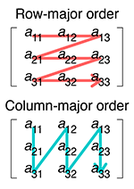
Row and column major order by Cmglee, CC BY-SA 4.0
The list of lists may have the rows separated in memory, they are written wherever
there is space. The arrays in numpy are guaranteed to be contiguous. The data
can be written across rows (row-major), or down the columns (col-major). To access
a value, internally numpy's code looks something like this:
val = arr[i * i_stride + j * j_stride];
For row-major data, i_stride = 1 and j_stride = n_columns. For col-major data
i_stride = n_rows and j_stride = 1. This can be extended into N dimensions
by adding further strides.
NB In R you can use the built-in array type, with any vector of dimensions dim. The indexing
is really intuitive and gives fast code. It's one of my favourite features of the
language. Note there is also a matrix type, which uses exactly two dimensions and silently
converts all entries to the same type -- use with care (particularly with apply, vapply is
often safer).
Why are numpy arrays faster?
- No type checking, as you're effectively using C code.
- Less pointer chasing as memory is contiguous (see compiled languages).
- Optimisations such as vectorised instructions are possible for the same reason.
- Functions to work with the data have been optimised for you (particularly linear algebra). And in some cases preallocation of the memory is faster than dynamically sized lists (though in python this makes less of a difference as lists are pretty efficient).
Simple matrix multiplication order in memory by Maxiantor, CC BY-SA 4.0
Let's compare summing values in a list of lists to summing a numpy array:
import numpy as np

def setup():
    xlen = 1000
    ylen = 1000

    rand_mat = np.random.rand(xlen, ylen)

    lol = list()
    for x in range(xlen):
        sublist = list()
        for y in range(ylen):
            sublist.append(rand_mat[x, y])
        lol.append(sublist)
    return rand_mat, lol

def sum_mat(mat):
    return np.sum(mat)

def sum_lol(lol):
    full_sum = 0
    for x in range(len(lol)):
        for y in range(len(lol[x])):
            full_sum += lol[x][y]
    return full_sum

def main():
    import timeit

    rand_mat, lol = setup()
    print(sum_mat(rand_mat))
    print(sum_lol(lol))

    setup_str = '''
import numpy as np
from __main__ import setup
from __main__ import sum_mat
from __main__ import sum_lol

rand_mat, lol = setup()
'''
    print(timeit.timeit("sum_mat(rand_mat)", setup=setup_str, number=100))
    print(timeit.timeit("sum_lol(lol)", setup=setup_str, number=100))

if __name__ == "__main__":
    main()
Which gives:
numpy sum: 500206.0241503447
list sum: 500206.0241503486

100x numpy sum time: 0.019256124971434474
100x list sum time: 9.559518916998059
A 500x speedup! Also note the results aren't identical, the implementations of sum cause slightly different rounding errors.
We can do a bit better using fsum:
def sum2_lol(lol):
    from math import fsum
    row_sum = [fsum(x) for x in lol]
    full_sum = fsum(row_sum)
    return full_sum
This takes about 2s (5x faster than the original, 100x slower than numpy) and gives a more precise result.
There are also advantages to preallocating memory space too, i.e. giving the size of the data first, then writing into the structure using appropriate indices. With the codon counting example, that might look like this:
def count_codons_numpy(seqs):
    # Precalculate codons and map them to integers
    bases = ['A', 'C', 'G', 'T']
    codon_map = dict()
    idx = 0
    for base1 in bases:
        for base2 in bases:
            for base3 in bases:
                codon = ''.join(base1 + base2 + base3)
                codon_map[codon] = idx
                idx += 1

    # Create a count matrix of zeros, and write counts directly into
    # the correct entry
    codon_len = int(len(seqs[0]) // 3)
    counts = np.zeros((codon_len, len(codon_map)), np.int32)
    for seq in seqs:
        for codon_idx in range(codon_len):
            codon = seq[codon_idx:(codon_idx + 3)]
            if not '-' in codon:
                counts[codon_idx, codon_map[codon]] += 1

    return counts
This is actually a bit slower than the above code as the codon_map means
accesses move around in memory rather than being to adjacent locations (probably
causing cache misses, but I haven't checked this.)
Sparse arrays
When you have numpy arrays with lots of zeros, as we do here, it can
be advantageous to use a sparse array. The basic idea is that rather than storing
all the zeros in memory, where we do have a non zero value (e.g. a codon count)
we store the value, its row and column position in the matrix. As well as saving
memory, some computations are much faster with sparse rather than dense arrays. They
are frequently used in machine learning applications. For example see lasso regression which can use a sparse array
as input, and jax for
use in deep learning.
You can convert a dense array to a sparse array:
sparse_counts = scipy.sparse.csc_array(counts)
print(sparse_counts)

  (3, 0)        4889
  (4, 0)        4889
  (5, 0)        4889
  (6, 0)        4889
  (81, 0)       4889
  (82, 0)       613
  (94, 0)       3281
...
In python you can use scipy.sparse.coo_array to build a sparse array, then convert it into csr or csc form
to use in computation.
In R you can use dgTMatrix,
and convert to dgCMatrix for computation. The glmnet package works well with this.
Just-in-time compilation
We mentioned above one of the reasons python code is not as fast as the numpy equivalent is due to the type checking that is needed when it is run. One way around this is with 'just-in-time compilation', where python bytecode is compiled to (fast) machine code at runtime and before a function executes, and checking of types is done once when the function is first compiled.
One package that can do this fairly easily is numba.
numba works well with simple numerical code like the sum above, but less well
with string processing, data frames or other packages. It can even run some code
on CUDA GPUs (I haven't tried it -- a quick look suggests it is somewhat fiddly but actually
quite feature-complete).
In many cases, you can run numba by adding an @njit decorator to your function.
NB I would always recommend using nopython=true or equivalently @njit as you otherwise you won't see when numba is failing to compile.
Exercise: Try running the sum_lol() and sum_lol2() functions using numba.
Time them. Run them twice and time each run. Note that fsum won't work, but you
can use sum. You will also want to use List from numba.
Expand the section below when you have tried this.
Sums with numba
import numpy as np
from numba import njit
from numba.typed import List

def setup():
    xlen = 1000
    ylen = 1000

    rand_mat = np.random.rand(xlen, ylen)

    lol = List()
    for x in range(xlen):
        sublist = List()
        for y in range(ylen):
            sublist.append(rand_mat[x, y])
        lol.append(sublist)
    return rand_mat, lol

@njit
def sum_mat(mat):
    return np.sum(mat)

@njit
def sum_lol(lol):
    full_sum = 0
    for x in range(len(lol)):
        for y in range(len(lol[x])):
            full_sum += lol[x][y]
    return full_sum

@njit
def sum2_lol(lol):
    row_sum = [sum(x) for x in lol]
    full_sum = sum(row_sum)
    return full_sum

def main():
    import timeit

    rand_mat, lol = setup()
    print(sum_mat(rand_mat))
    print(sum_lol(lol))

    setup_str = '''
import numpy as np
from __main__ import setup
from __main__ import sum_mat, sum_lol, sum2_lol

rand_mat, lol = setup()

# Compile the functions here
run1 = sum_mat(rand_mat)
run2 = sum_lol(lol)
run3 = sum2_lol(lol)
'''
    print(timeit.timeit("sum_mat(rand_mat)", setup=setup_str, number=100))
    print(timeit.timeit("sum_lol(lol)", setup=setup_str, number=100))
    print(timeit.timeit("sum2_lol(lol)", setup=setup_str, number=100))

if __name__ == "__main__":
    main()
This now gives the same result between both implementations:
500032.02596789633
500032.02596789633
and the numba variant using the built-in sum is a similar speed to numpy (time in s):
sum_mat 0.09395454201148823
sum_lol 2.7725684169563465
sum2_lol 0.08274500002153218
We can also try making our own array class with strides rather than using lists of lists:
@njit
def sum_row_ar(custom_array, x_size, x_stride, y_size, y_stride):
    sum = 0.0
    for x in range(x_size):
        for y in range(y_size):
            sum += custom_array[x * x_stride + y * y_stride]
    return sum
This about twice as fast as the list of list sum (1.4s), but still a lot slower than the built-in sums which can benefit from other optimisations.
Working with characters and strings
Needing arrays of characters (aka strings) is very common in sequence analysis, particularly with genomic data. It's very easy to work with strings in python (less so in R), but not always particularly fast. If you need to optimise string processing ultimately you may end up having to use a compiled language -- we will work through an example counting substrings (k-mers) from sequence reads in a later chapter.
That being said, numpy does have some support for working with strings by treating
them as arrays of characters. Characters are usually
coded as ASCII, which
uses a single byte (8 bits: np.int8/u8/char/uint8_t depending on language).
Note that unicode, which is crucially needed for encoding emojis 🕴️ 🤯 🐈⬛ 🦉 and therefore essential to any modern research code, is a little more complex as it is variable length and uses an terminating character.
We can read our string directly into a numpy array of bytes as follows:
s = np.frombuffer(s.lower().encode(), dtype=np.int8)
Genome data often has upper and lowercase bases (a or A, c or C and so on) with no particular meaning assigned to this difference. It's useful to convert everything to a single case for consistency.
Here is an example converting the bases {a, c, g, t} into {0, 1, 2, 3}/{b00, b01, b10, b11}
and using some bitshifts to do the codon counting:
@njit
def inc_count(codon_map, X):
    for idx, count in enumerate(codon_map):
        X[count, idx] += 1

def count_codons(seqs, n_codons):
    n_samples = 0
    X = np.zeros((65, n_codons), dtype=np.int32)
    for s in seqs:
        n_samples += 1
        s = np.frombuffer(s.lower().encode(), dtype=np.int8).copy()
        # Set ambiguous bases to a 'bin' index
        ambig = (s!=97) & (s!=99) & (s!=103) & (s!=116)
        if ambig.any():
            s[ambig] = 64
        # Shape into rows of codons
        codon_s = s.reshape(-1, 3).copy()
        # Convert to usual binary encoding
        codon_s[codon_s==97] = 0
        codon_s[codon_s==99] = 1
        codon_s[codon_s==103] = 2
        codon_s[codon_s==116] = 3
        # Bit shift converts these numbers to a codon index
        codon_s[:, 1] = np.left_shift(codon_s[:, 1], 2)
        codon_s[:, 2] = np.left_shift(codon_s[:, 2], 4)
        codon_map = np.fmin(np.sum(codon_s, 1), 64)
        # Count the codons in a loop
        inc_count(codon_map, X)

    # Cut off ambiguous
    X = X[0:64, :]

    return X, n_samples
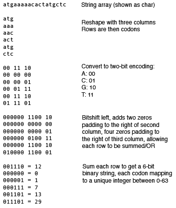 Overview of the algorithm
This also checks for any non-acgt bases and puts them in an imaginary 65th codon,
which acts as a bin for any unobserved data. Stops can also be removed. A numba
loop is used to speed up the final count.
Overall this is about 50% faster than the dictonary implementation for this size of data, but is quite a bit more complex and likely error-prone. This type of processing can become worth it when the strings are larger, as we will see.
Alternative python implementations
We can also try alternative implementations of the python interpreter over the
standard CPython. A popular one is pypy which can
be around 10x faster for no extra effort. You can install via conda.
On my system for the sum benchmake, this ended up being 3-10x slower than CPython:
sum_lol 36.7518346660072
sum2_lol 56.79283958399901
but for the codon counting benchmark, was about twice as fast:
fn1: 2.63s
fn2: 0.83s
It costs almost nothing to try in many cases, but make sure you take some measurements.
Memory optimisation
It's often the case that you want to reduce memory use rather than increase speed. Similar tools can be used for memory profiling, however in python this is more difficult. If memory is an issue, using a compiled language where you have much more control over allocation and deallocation, moving and copying usually makes sense.
In python, using preallocated arrays can help you control and predict memory, and ensuring you don't copy large objects or delete them after use is also a good start.
Some other tips:
- Avoid reading everything into memory and compute 'on the fly'. The above code reads in all of the sequences first, then processes them one at a time. These could be combined, so codons counts are updated after each sequence is read in, so then only one sequence needs to fit in memory.
- You can use disk (i.e. files) to move objects in and out of memory, at the cost of time.
- Memory mapping large files you wish to modify part of can be an effective approach.
Writing extensions in compiled code
It is possible to write C/C++ code and call it from python using Cython. Instead,
I would highly recommend either the pybind11
or nanobind packages which make this a lot easier.
The tricky part is writing your setup.py and Makefile/CMakeLists.txt to get
everything to work together. If you are interested in this approach, examples from
some of our group's packages may be helpful:
sketchlibcalls C++ and CUDA code from python.mandrakedoes the same, but also returns an object used in the python code.ggcalleruses both python and C++ code throughout.
Please feel free to adapt and reuse the build approach taken in any of these.
Other optimisations
For data science, have a look at the following packages for tabular data:
cuDF- GPU accelerated data frames: https://docs.rapids.ai/api/cudf/stable/- Apache arrow and Parquet format: https://arrow.apache.org/docs/python/index.html
Notes (for next year)
- Code should probably be given, rather than written
- This isn't doable for R users
- 1st part unclear what should be read/checked
- Which reading frames
- Snakeviz a good tool for visualisation of profiles
- Better examples of fasta and expected output
- Bitshift example is the wrong way round
HPC
In this session we will look at running code on compute clusters.
An initial consideration is always going to be 'when should I run code on the cluster rather than my laptop?'. I think the following are the main reasons:
- Not enough resources on your machine (e.g. not enough memory, needs a high-end GPU).
- Job will take longer than you want to leave you machine on for.
- Running many jobs in parallel.
- Using data which is more easily/only accessed through cluster storage.
- A software installation which works more easily on cluster OS (e.g. linux rather than OS X).
- Benchmarking code.
Of course it's almost always easier to run code on your local machine if you can avoid these cases. Weighing up effort to run on the HPC versus the effort of finding workarounds to run locally is hard. Making the HPC as painless as possible, while acknowledging there will always be some pain, is probably the best approach.
Particular pain-points of using the HPC can be:
- Clunky interface, terminal only.
- Waiting for your jobs to run.
- Running jobs interactively.
- Installing software.
- Troubleshooting jobs or getting code to run.
- Running many jobs at once and resubmitting failed jobs.
- Making your workflow reproducible.
I've tried to present solutions to these in turn, including three exercises:
- Estimating resource use.
- Installing software without admin rights.
- Running a job array.
Some of this will be specific to the current setup of the EBI codon cluster. I'm sticking with LSF for now -- a change to SLURM is planned because apparently it has better metrics centrally. Similar principles apply as with LSF, some features do change. For this year cloud computing won't be covered (sorry), but I can try and add this in future. So the topics for today:
- Maximising your quality of life on the HPC
- LSF basics (recap)
- Getting jobs to run and requesting resources
- Interactive jobs
- Installing software without admin rights
- Troubleshooting jobs and prototyping code
- Job arrays
- Reproducibility on the HPC
Maximising your quality of life on the HPC
There are some basic tools you can use for bash/zsh and Unix which will make your time on the HPC less unpleasant. I'll mention them here -- if they look useful try them out after the class.
If anyone has further suggestions, now is a good time to discuss them.
tmux
This is my biggest piece of advice in this section: always use tmux to maintain
your session between log ins. (You may have used screen before, tmux has more
features and is universally available).
The basic usage is:
- When you log in for the first time, type
tmux new(ortmux new zshif you wanted to run a specific terminal). - This is your session, run commands as normal within the interface.
- When it's time to log out, press
Ctrl-bthend(for detach). - Next time you log in, type
tmux attachto return to where you were. - Use
Ctrl-bthencto make a new tab.Ctrl-band a number or arrow to switch between. - Use
Ctrl-bthen[then arrows to scroll (but easier to make this the mouse as normal through config file).
If you crash/lose connection the session will still be retained. Sessions are lost
when the node reboots. Also note, you need to specify a specific node e.g. codon-login-01
rather than the load-balancer codon-login when using tmux.
There are many more features available if you edit the ~/.tmux.conf file. In particular
it's useful to turn the mouse on so you can click between panes and scroll as normal.
Here's an old one of mine with more
examples.
Background processes
Less useful on a cluster, but can be if you ever use a high-performance machine without a queuing system (e.g. openstack, cloud).
Ctrl-z suspends a process and takes you back to the terminal. fg to foreground (run
interactively), bg to keep running but keep you at the prompt. See jobs to look
at your processes.
You can add an ampersand & at the end of a command and it will run in the background
without needing to suspend first. nohup will keep running even when you log out
(not necessary if you are using tmux).
Text editors
Pick one of vi/vim/gvim/neovim or emacs and learn some of the basic commands.
Copying and pasting text, find and replace, vertical editing and repeating custom commands
are all really useful to know. Once you're used to them, the extensions for VSCode which
let you use their commands are very powerful.
Although, in my opinion, they don't replace a modern IDE such as VSCode every system has them installed and it's very useful to be able to make small edits to your code or other files. Graphical versions are also available.
Terminal emulators
Impress your friends and make your enemies jealous by using a non-default terminal emulator. Good ones:
zsh and oh-my-zsh
I personally prefer zsh over bash because:
- History is better. Type the start of a command, then press up and you'll get the commands you've previously used that started like that. For example, type
lsthen press up. - The command search
Ctrl-Ris also better. - Keep pressing tab and you'll see options for autocomplete.
I'm sure there are many more things possible.
zsh is now the default on OS X. You can change shell with chsh, but you usually
need admin rights. On the cluster, you can just run zsh to start a new session,
but if you're using tmux you'll pop right back into the session anyway.
You can also install oh-my-zsh which has some nice extensions, particularly for within git directories. The little arrow shows you whether the last command exited with success or not.
Enter-Enter-Tilde-Dot
This command exits a broken ssh session. See here for more ssh commands.
Other handy tools I like
agrather thangrep.fdrather thanfind.fzffor searching through commands. Can be integrated withzsh.
While I'm writing these out, can't resist noting one of my favourite OS X commands:
xattr -d "com.apple.quarantine" /Applications/Visual\ Studio\ Code.app
Which gets rid of the stupid lock by default on most executables on OS X.
LSF basics (recap)
- Submit jobs with
bsub. - Check your jobs with
bjobs.bjobs -dto include recently finished jobs. - View the queues with
bqueues. Change jobs withbswitch. bstop,bresume,brestartto manage running jobs. End jobs withbkill.bhostsandlshoststo see worker nodes.bmodto change a job.
Most of these you can add -l to get much more information. bqueues -l is interesting
as it shows your current fair-share priority (lower if you've just run a lot of jobs).
There are more, but these are the main ones. Checkpointing doesn't work well, as far as I know.
Getting jobs to run and requesting resources
It's frustrating when your jobs take a long time to run. Requesting the right amount of resources both helps your job find a slot in the cluster to run, and lowers the load overall helping everyone's jobs to run.
That being said, I don't want to put anyone off experimenting or running code on the HPC. Don't worry about trying things out or if you get resource use wrong. Over time improving your accuracy is worthwhile, but it's always difficult with a new task -- very common in research! We now have some nice diagnostics and history here I'd recommend checking out periodically to keep track of how you're doing: http://hoxa.windows.ebi.ac.uk:8080/.
The basic resources for each CPU job are:
- CPU time (walltime)
- Number of CPU cores
- Memory
/tmpspace
Though the last of these isn't usually a concern, we have lots of fast scratch space you can point to if needed. Disk quotas are managed outside of LSF and I won't discuss them here.
When choosing how much of these resources to request, you want to avoid:
- The job failing due to running out of resources.
- Using far less than the requested resources.
- Long running jobs.
- Inefficient resource use (e.g. partial parallelisation, peaky maximum memory).
- Requesting resources which are hard to obtain (many cores, long run times, lots of memory, lots of GPUs).
- Lots of small jobs.
- Inefficient code.
Typically 1) is worse than 2). Those resources were totally wasted rather than partially wasted. We will look at this in the exercise.
Long running jobs are bad because failure comes at a higher cost, and it makes the cluster use less able to respond to dynamic demand. Considering adding parallelisation rather than a long serial job if possible, or adding some sort of saving of state so jobs can be resumed.
You can't usually do much about the root causes of 4) unless you wrote the code yourself. You will always need a memory request which is at least the maximum demand (you can have resource use which changes over the job, but it's not worth it unless e.g. you are planning the analysis of a biobank). Inefficient parallel code on a cluster may be better as a serial job. Note that if you don't care about the code finishing quickly it's always more efficient in CPU terms to run them on a single core. For example, if you have 1000 samples which you wished to run genome assembly on would you run:
- 1000 single-threaded jobs
- 1000 jobs with four threads
- 1000 jobs with 32 threads?
(we will discuss this)
-
can sometimes be approached by using job arrays or trading off your requests. Sometimes you're just stuffed.
-
is bad because of the overhead of scheduling them. Either write a wrapper script to run them in a loop, or use the
shortqueue. -
at some point it's going to be worth turning your quickly written but slow code into something more efficient, as per the previous session. Another important effect can come from using the right compiler optimisations, which we will discuss next week.
Anatomy of a bsub
Before the exercise, let's recap a typical bsub command:
bsub -R "select[mem>10000] rusage[mem=10000]" -M10000 \
-n8 -R "span[hosts=1]" \
-o refine.%J.o -e refine.%J.e \
python refine.py
-R "select[mem>10000] rusage[mem=10000]" -M10000requests ~10Gb memory.-n8 -R "span[hosts=1]"requests 8 cores on a single worker node.-o refine.%J.o -e refine.%J.ewrites STDOUT and STDERR to files named with the job number.python refine.pyis the command to run.
NB the standard memory request if you don't specify on codon is 15Gb. This is a lot, and you should typically reduce it.
If you want to capture STDOUT without the LSF header add quotes:
bsub -o refine.%J.o -e refine.%J.e "python refine.py > refine.stdout"
You can also make execution dependent on completion of other jobs with the -w flag
e.g. bsub -w DONE(25636). This can be useful in pipeline code.
When I first started using LSF I found a few commands helpful for looking through your jobs:
bjobs -a -x
find . -name "\*.o" | xargs grep -L "Successfully completed"
find . -name "\*.o" | xargs grep -l "MEMLIMIT"
find . -name "\*.e" | xargs cat
Exercise 1: Estimating resource use
You submit your job, frantically type bjobs a few times until you see it start
running, then go off and complete the intermediate programming class feedback form while you wait. When you check
again, no results and a job which failed due to running out of memory, or going over run time. What now?
You can alter your three basic resources as follows:
- CPU time: ask for more by submitting to a different queue.
- CPU time: use less wall time by asking for more cores and running more threads.
- Memory: ask for more in the
bsubcommand.
Ok, but how much more? There are three basic strategies you can use:
- Double the resource request each time.
- Run on a smaller dataset first, then estimate how much would be needed based on linear or empirical scaling.
- Analyse the computational efficiency analytically (or use someone else's analysis/calculator).
The first is a lazy but effective approach for exploring a scale you don't know the maximum of. Maybe try this first, but if after a couple of doublings your job is still failing it's probably time to gather some more information.
Let's try approach two on a real example by following these steps:
- Find the sequence alignment from last week. Start off by cutting down to just the first four sequences in the file.
- Install RAxML version 8. You can get the source here, but it's also more easily available via bioconda.
- Run a phylogenetic analysis and check the CPU and memory use. The command is of the form
raxmlHPC-SSE3 -s BIGSdb_024538_1190028856_31182.dna.aln -n raxml_1sample -m GTRGAMMA -p 1. - Increase the number of samples and retime. I would suggest a log scale, perhaps doubling the samples included each time. Plot your results.
- Use your plot to estimate what is required for the full dataset.
If you have time, you can also try experimenting with different numbers of CPU threads (use the PTHREADS version and -T), and number of sites
in the alignment too.
You can use codon or your laptop to do this.
LSF is really good at giving you resource use. What about on your laptop? Using
/usr/bin/time -v (gtime -v on OS X, install with homebrew) gives you most of the same information.
What about approach three? (view after exercise)
For this particular example, the authors have calculated how much memory is required and even have an online calculator. Try it here and compare with your results.
Adding instrumentation to your code
We said in optimisation that some measurement is better than no measurement.
I am a big fan of progress bars. They give a little more information than just the total time and are really easy to add in. When you've got a function that just seems to hang, seeing the progress and expected completion time tells you whether your code is likely to finish if you just wait a bit longer, or if you need to improve it to have any chance of finishing. This also gives you some more data, rather than just increasing the wall time repeatedly.
In python, you can wrap your iterators in tqdm which gives you a progress bar
which number of iterations done/total, and expected time.
tqdm progress bars in python
GPUs
I have not used the GPUs on the codon cluster, but a few people requested that I cover them.
In the session I will take a moment if anyone has experience they would like to discuss.
The following are a list of things I think are relevant from my use of GPUs (but where I have admin rights and no queue):
- Use
nvidia-smito see available GPUs, current resource use, and driver version. - Using multiple GPUs is possible and easier if they are the same type.
- GPUs have a limited amount device memory, usually around 4Gb for a typical laptop card to 40Gb for a HPC card.
- The hierarchy of processes is: thread -> warp (32 threads) -> block (1-16 warps which share memory) -> kernel (all blocks needed to run the operation) -> graph (a set of kernels with dependencies).
- Various versions to be aware of: driver version (e.g. 410.79) -- admin managed; CUDA version (e.g. 11.3) -- can be installed centrally or locally; compute version (e.g. 8.0 or Ampere) -- a feature of the hardware. They need to match what the package was compiled for.
- When compiling, you will use
nvccto compile CUDA code and the usual C/C++ compiler for other code.nvccis used for a first linker step, the usual compiler for the usual final linker step. pytorchetc have recommended install routes, but if they don't work compiling yourself is always an option.- You can use
cuda-gdbto debug GPU code. Use is very similar togdb. Make sure to compile with the flags-g -G. - Be aware that cards have a maximum architecture version they support. This is the compute version given to the CUDA compiler as sm_XX. For A100 cards this is sm_80.
See here for some relevant installation documentation for one of our GPU packages: https://poppunk.readthedocs.io/en/latest/gpu.html
Using GPUs for development purposes? We do have some available outside of codon which are easier to play around with.
Interactive jobs
Just some brief notes for this point:
- Use
bsub -I, and without the-oand-eoptions to run your job interactively, i.e. so you are sent to the worker node terminal as the job runs. - Make sure you are using X11 forwarding to see GUIs. Connect with
ssh -X -Y <remote>, and you may also need Xquartz installed. - If you are using
tmuxyou'll need to make sure you've got the right display. Runecho $DISPLAYoutside of tmux, thenexport DISPLAY=localhost:32(with whatever$DISPLAYcontained) inside tmux. - If you want to view images on the cluster without transferring files, you can
use
display <file.png> &. For PDFs see here.
Ultimately, it's a pain, and using something like OpenStack or a VM in the cloud is likely to be a better solution.
Installing software without admin rights
If possible, install your software using a package manager:
homebrewon OS X.apton Ubuntu (requires admin).conda/mambaotherwise.
conda tips
-
Install miniconda for your system.
-
Add channels in this order:
    conda config --add channels defaults
    conda config --add channels bioconda
    conda config --add channels conda-forge
- If you've got an M1 Mac, follow this guide to use Intel packages.
- Never install anything in your base environment.
- To create a new environment, use something like
conda create env -n poppunk python==3.9 poppunk. - Environments are used with
conda activate poppunkand exited withconda deactivate. - Create a new environment for every project or software.
- If it's getting slow at all, use
mambainstead! Use micromamba to get started. - Use
mambafor CI tasks. - You can explicitly define versions to get around many conflicts, in particular changing the python version is not something that will be allowed unless explicitly asked for.
- For help: https://conda-forge.org/docs/user/tipsandtricks.html.
Also note:
- anaconda: package repository and company.
- conda: tool to interact with anaconda repository.
- miniconda: minimal version of the anaconda repostory and conda.
- conda-forge: general infrastructure for creating open-source packages on anaconda.
- bioconda: biology-specific version of conda-forge.
- mamba: a different conda implementation, faster for resolving environments.
What about if your software doesn't have a conda recipe? Consider writing one! Take
a look at an example on bioconda-recipes and copy it to get started.
Exercise 2: Installing a bioinformatics package
Let's try and install bcftools.
To get the code, run:
git clone --recurse-submodules https://github.com/samtools/htslib.git
git clone https://github.com/samtools/bcftools.git
cd bcftools
The basic process for installing C/C++ packages is:
./configure
make
make install
You can also usually run make clean to remove files and start over, if something goes wrong.
Typically, following this process will try and install the software for all users in the system directory /usr/local/bin
which you won't have write access to unless you are root (admin). Usually the workaround is to
set PREFIX to a local directory. Make a directory in your home called software mkdir ~/software and
then run
./configure --prefix=$(realpath ~/software)
make && make install
This will set up some of your directories in ~/software for you. Other directories
you'll see are man/ for manual pages and lib/ for shared objects used by many
different packages (ending .so on Linux and .dylib on OS X).
If there's no --prefix option for the configure script, you can often override
the value in the Makefile by running:
PREFIX=$(realpath ~/software) make
The last resort is to edit the Makefile yourself. You can also change the optimisation
options in the Makefile by editing the CFLAGS (CXXFLAGS if it's a C++ package):
CFLAGS=-O3 -march=native make
Compiles with the top optimisation level and using instructions for your machine.
Try running bcftools -- not found. You'll need to add ~/software to your PATH
variable, which is the list of directories searched by bash/zsh when you type a command:
export PATH=$(realpath ~/software)${PATH:+:${PATH}}
To do this automatically every time you start a shell, add it to your ~/.bashrc or ~/.zshrc file.
Try running make test to test the installation.
To use the bcftools polysomy command requires the GSL library. Install that next. Ideally you'd just use your package manager, but let's do it
from source:
wget https://ftp.gnu.org/gnu/gsl/gsl-latest.tar.gz
tar xf gsl-latest.tar.gz
./configure --prefix=/Users/jlees/software
make -j 4
make install
Adding -j 4 will use four threads to compile, which is useful for larger projects.
Your software/ directory will now has an include/ directory where headers needed
for compiling/making with the library are stored, and a lib/ directory with
libraries needed for running software with the library are stored.
We need to give these to configure:
./configure --prefix=/Users/jlees/software --enable-libgsl CFLAGS=-I/Users/jlees/software/include LDFLAGS=-L/Users/jlees/software/lib
make
Finally, to run bcftools the gsl library also needs to be available at runtime (as opposed
to compile time, which we ensured by passing the paths above). You can
check which libraries are needed and if/where they are found with ldd bcftools (otool -L on OS X):
bcftools:
        /usr/lib/libz.1.dylib (compatibility version 1.0.0, current version 1.2.11)
        /usr/lib/libSystem.B.dylib (compatibility version 1.0.0, current version 1319.100.3)
        /usr/lib/libbz2.1.0.dylib (compatibility version 1.0.0, current version 1.0.8)
        /usr/lib/liblzma.5.dylib (compatibility version 6.0.0, current version 6.3.0)
        /usr/lib/libcurl.4.dylib (compatibility version 7.0.0, current version 9.0.0)
        /Users/jlees/software/lib/libgsl.27.dylib (compatibility version 28.0.0, current version 28.0.0)
        /System/Library/Frameworks/Accelerate.framework/Versions/A/Frameworks/vecLib.framework/Versions/A/libBLAS.dylib (compatibility version 1.0.0, current version 1.0.0)
So libgsl.dylib and libBLAS.dylib are being found ok. If they aren't being found, you need
to add ~/software/lib to the LD_LIBARY_PATH environment variable like you did with the PATH.
Check that you can run bcftools polysomy.
Troubleshooting jobs and prototyping code
Some tips:
- It's ok to run small jobs on the head node, especially to check you've got the arguments right. Then kill them with
Ctrl-Corkillonce they get going. Avoid running things that use lots of memory (these will likely be killed automatically). You can preface your command withniceto lower its priority. - Find a smaller dataset which replicates your problems, but gets to them without lots of CPU and memory use. Then debug interactively rather than through the job submission system.
- Run a simple or example analysis first, before using your real data or the final set of complex options.
- Add print statements through your code to track where the problem is happening.
- If that doesn't find the issue, use a debugger interactively (see last session). For compiled code giving a segfault, this is usually the way to fix it (or with
valgrind). - If you need to debug on a GPU, be aware this will stop the graphics output.
- Try and checkpoint larger tasks. Save temporary or partial results (in python with a pickle, in R with
saveRDS). Pipeline managers will help with this and let you resume from where things went wrong. - Split your task into smaller jobs. For example, if you have code which parses genomic data into a data frame, runs a regression on this data frame, then plots the results. Split this into three scripts, each of which saves and loads the results from the previous step (using serialisation).
Job arrays
If you have embarrasingly parallel tasks, i.e. those with no shared memory or dependencies, job arrays can be an incredibly convenient and efficient way to manage batching these jobs. Running the same code on multiple input files is a very common example. In some settings, using a job array can give you higher overall priority.
To use an array, add to your bsub command:
bsub -J mapping[1-1000]%200 -o logs/mapping.%J.%I.o -e logs/mapping.%J.%I.e ./wrapper.py
-Jgives the job a name[1-1000]gives the index to run over. This can be more complex e.g.[1,2-20,43], useful for resubmitting failed jobs.%200gives the maximum to run at a time. Typically you don't need this because the scheduler will sort out priority for you, but if, for example, you are using a lot of temporary disk space for each job it may be useful to restrict the total running at any given moment.- We add
%Ito the output file names which is replaced with the index of the job so that every member of the array writes to its own log file.
The key thing with a job array is that an environment variable LSB_JOBINDEX will be
created for each job, which can then be used by your code to set up the process correctly.
Let's work through an example.
Exercise 3: Two-dimensional job array
Let's say I have the following python script which does a stochastic simulation of an infectious disease outbreak using an SIR model and returns the total number of infections at the end of the outbreak:
import numpy as np

def sim_outbreak(N, I, beta, gamma, time, timestep):
    S = N - I
    R = 0
    max_incidence = 0
    n_steps = round(time/timestep)

    for t in range(n_steps):
        infection_prob = 1 - np.exp(-beta * I / N * timestep)
        recovery_prob = 1 - np.exp(-gamma * timestep)

        number_infections = np.random.binomial(S, infection_prob, 1)
        number_recoveries = np.random.binomial(I, recovery_prob, 1)

        S += -number_infections
        I += number_infections - number_recoveries
        R += number_recoveries

    return R

def main():
    N = 1000
    I = 5
    time = 200
    timestep = 0.1
    repeats = 100

    beta_start = 0.01
    beta_end = 2
    beta_steps = 100

    gamma_start = 0.01
    gamma_end = 2
    gamma_steps = 100

    for beta in np.linspace(beta_start, beta_end, num=beta_steps):
        for gamma in np.linspace(gamma_start, gamma_end, num=gamma_steps):
            sum_R = 0
            for repeat in range(repeats):
                sum_R += sim_outbreak(N, I, beta, gamma, time, timestep)
            print(f"{beta} {gamma} {sum_R[0]/repeats}")

if __name__ == "__main__":
    main()
The main loop runs a parameter sweep over 100 values of beta and gamma (so \(10^4\) total), and runs 100 repeats (so \(10^6\) total). Each of these parameter combinations takes around 3s to run on my machine, so we'd be expecting about 8 hours total. We could of course use some tricks from last week to improve these, but instead lets use a job array to parallelise.
Do the following:
- Change the
beta_stepsandgamma_stepsto 5 (so we don't all hammer the cluster too hard). - Use
import osandjob_index = os.environ['LSB_JOBINDEX']to get the job index at the start of the main function. - Replace the outer loop over beta with this index, so that the job runs a single beta value, but the full loop over gamma.
- Write an appropriate
bsubcommand to submit this is a job array. Use the-q shortqueue. - Think about how you would collect the results from all of your jobs (using either bash or by modifying the code).
If you have time:
- Also replace the gamma loop, so that each job in the array (of 25 jobs) runs just a single beta and gamma value, but the full repeat loop.
- Change the print statement so it's easier to collect your results at the end.
It may help to review the section on strides from the previous session when you are thinking about how to map a 1D index into two dimensions.
One other note: here we are using random number generators across multiple processes. If they have the same seed, which may be the default, they will produce identical results and likely be invalid repeats. Even if they are set to different seeds (either by using the job index or by using the system clock), after some time they will likely become correlated, which may also cause problems. See Figure 3 in this paper for how to fix this.
Reproducibility on the HPC
Tips based on what has worked for me:
- Keeping track of your command history goes a long way. Set up your history options with unlimited scrollback and timestamps.
- Search through history in the following order:
- Type the start of your command, then press up.
- Use Ctrl-r to search for part of your command.
- Use
history | grepfor more complex searches. e.g.history | grep sir.py | grep bsubwould find when thesir.pyscript was submitted with bsub. You can use-Cto add context and see other commands. Or usehistory | lessand the search function to find the sequence of commands you used.
- Be careful with editing files in a text editor on the cluster -- this command cannot just be rerun and it won't be clear what you did.
- Use git for everything you write, and commit often.
- For larger sets of jobs, particularly which you will run repeatedly or expect some failures, it may be worth using pipeline software (snakemake, nextflow) to connect everything together. Ususally they can handle the
bsub/SLURM submission for you. - Keep your code and data separate.
- Don't modify your input data, instead make intermediate files.
- Don't overwrite files unless you have to. Regularly clean and tidy files you are working on.
- Call your files and directories sensible names and write a
READMEif they get complicated. - Think about your main user: future you. Will you be able to come back to this in a month's time? Three year's time?
- Use
-oand-ewith all jobs, and write tologs/folders. You can easilytarthese once you are done. - Make plots on your local machine (with code that can be run through without error or needing the current environment). Transfer smaller results files from the HPC to make your plots.
- Use conda environments to make your software versions consistent between runs. Use
conda listto get your software and versions when you write papers.
Compiled languages
Before starting this session please review the prerequisites. You should at least have the rust toolchain installed.
In this module you will be introduced to a compiled language called rust. There are three parts:
a. Introduction (this session). A description of basics in rust. No main exercise.
b. Data structures. A description of some more complex types in rust. Exercise: k-mer counter.
c. Object-oriented programming. Using objects (structs) to write your code. Exercise: Gaussian blur.
Some other examples of compiled languages include C, C++ and Fortran. I've chosen rust mostly because of its great build system. It's much easier to set up than other compilers, which would be a multi-hour session in its own right. The syntax is not massively dissimilar from python and there are good third party packages available. I expect that more research software projects will use it in the future.
Languages like R, python and Julia are interpreted languages. Roughly what this means
is that every time you run the code, it is first translated into machine code which is
what the computer actually runs, and then run. You can think of the translation
and run happening for each time you get to a new line. (NB: We've also looked at packages like numba which could compile a single
function in python).
In a compiled language, these two steps are split up. Before running the program, you run a compiler on all of your code (known as compile-time), which converts it into machine code and creates an executable. Each time you run the code (known as run-time), you then directly run the executable without having to compile the code. Clearly this can be more efficient, but why else might you want to use a compiled language:
- Speed. As well as skipping the interpreting step, the compiler being able to see all the code at once can automatically optimise your code. Knowing the types of all the variables also avoids other expensive checks. For CPU intensive tasks, it's not unreasonable to expect 10x or more faster code by default.
- Control of memory. Compiled languages allow you to pass objects by copying them, moving them, or by passing a reference. This more direct interface to shared memory gives much more control of data, which can be crucial when working with large arrays.
- Easier/better parallelisation. Similar to memory, the extra control typically allows multiprocessing to be a lot more efficient, and it is often easier to implement.
- Type checking. As we will see, all variables must have a type, for example integer, string, or float. Beyond just speed, ensuring these are compatible can catch errors at compile-time.
- Shipping a binary. It is possible to include everything you need to run your code in a single file. No need for conda, and updated libraries with different APIs won't break your code.
Sounds great! So why isn't everything written in compiled languages? I would say the two main reasons are that:
- It is fundamentally a bit more complicated to learn and write code in a compiled language, so it takes longer to develop in.
- R and python are really popular and have loads of great packages to use -- often you end up implementing more yourself in a compiled language.
In this session we will:
- Introduce the basics of rust and its build system, and write some simple example code.
- Review some of the practical aspects of writing rust code: debugging, profiling and optimising.
The next part of the session will then take your rust skills further, and we will look at some common data structures you can use to accelerate your compiled code. Finally, we will work through an example using object oriented programming to implement Gaussian blur on images.
We only have time for a short introduction, but if this piques your interest the 'Rust By Practice' book is a good place to continue.
Please note that you can actually run the rust code in the examples here if you press the play button.
General introduction
Compiling code
To make a new rust project, run:
cargo new iprog
This will create a new project called 'iprog'. Change into that directory and
you will see Cargo.toml, which contains the metadata about your project, and
the src/ directory for the code. This currently contains main.rs which is
the source for your program. It is of course possible to split this over multiple
files or make libraries rather than executables, but this is beyond the scope of this
course, and we will just use this simple structure throughout.
The Cargo.toml lets you set the version of your code, other information such
as the authors. It's also where you list any dependencies, which we will use later on.
The default main.rs contains a simple program which writes 'Hello, world!' to
the terminal when run. The main() function is what is run when the code starts,
and println means 'print line'. The ! is a macro, a special shorthand for
some common functions:
fn main() {
    println!("Hello, world!");
}
(try running this with the 'play' button)
Some other commands you'll need for running your code are:
cargo run
Try this in your code directory. You'll see that the code is compiled, and then run.
If you want to compile the code run:
cargo build
You'll then get an executable in target/debug/iprog. Try running that directly.
Why is it under debug/? As noted above, when we compile this code the compiler itself can make
various optimisations which make the code run faster. For example, eliminating unused
sections of code, combining instructions, guessing which branch of the loop is
likely to be executed. However, this means the executed code doesn't always correspond
to lines in your source. When run with debug mode on (which is the default) most optimisations
are turned off to help you step through the code line by line. But when you are ready
to test the 'proper' version of your code, instead you add the --release flag:
cargo build --release
    Finished release [optimized] target(s) in 0.22s
You'll see this says optimized and you can run it from target/release/iprog.
Have a look at https://godbolt.org/ if you want to see how source code translates
to machine code under different levels of optimisation.
Finally, if you want to install your program, so you can run it just by typing iprog
at the command prompt, run:
cargo install --path .
Note that the default is to compile the optimised code for the installed version.
More useful commands:
cargo fmtwill format your code nicely.cargo clippyruns the linter.cargo testruns any tests you have written.
Types
One of the most important distinctions between languages is how they deal with the types of their variables. Rust is 'strongly typed' and 'statically typed', which means that all variables have to have known types at compile time, and trying to assign between different types will result in a compiler error.
In rust, you use the let keyword to define a variable:
#![allow(unused)]
fn main() {
let number = 64;
println!("{number}");
}
Here, rust has automatically inferred the type of number, but we can set it
explicitly to the integer type i32 (which we will explain in a moment) as follows:
#![allow(unused)]
fn main() {
let number: i32 = 64;
println!("{number}");
}
Let's try comparing an integer to a floating point f64:
#![allow(unused)]
fn main() {
let int: i32 = 64;
let decimal: f64 = 64.0;
if int == decimal {
    println!("Equal");
} else {
    println!("Unequal");
}
}
This gives a compiler error:
5 | if int == decimal {
  |    ---    ^^^^^^^ expected `i32`, found `f64`
  |    |
  |    expected because this is `i32`
We cannot assign or compare between two different types. But if we convert the
integer to a float using as, this will work:
#![allow(unused)]
fn main() {
let int: i32 = 64;
let floaty_int = int as f64;
let decimal: f64 = 64.0;
if floaty_int == decimal {
    println!("Equal");
} else {
    println!("Unequal");
}
}
A brief overview of the types in rust which are most likely to useful for you:
| Type | Description |
|---|---|
i32 | Signed integer using 32-bits, range -2,147,483,648 to 2,147,483,647. Equivalent to int or long in C++, int in python, int in R. |
u32 | Unsigned (i.e. positive) integer using 32-bits, range 0 to 4,294,967,295. |
usize | Used for sizes/lengths (e.g. length of a list), positive numbers only. |
f64 | Floating point (decimal) number stored using 64-bits. Equivalent to double in C++, float in python, num in R |
char | A Unicode character such as 'a', 'é' or '🫠'. |
bool | A boolean, true or false. |
Vec | A vector, which is the name for a list/array where the size can change. |
String | A string, which is effectively a list unicode characters (not quite a Vec of char, but similar). You may also see str passed to functions, which is the same, except isn't 'owned' so the length can't be changed. |
Tuples can be written and accessed as follows:
#![allow(unused)]
fn main() {
let tuple: (i32, char, bool) = (500, 'b', true);
println!("{} {} {}", tuple.0, tuple.1, tuple.2);
}
The .0 means the 1st element (rust is 0-indexed, same as python, different to R). Note
also that in the println! any empty brackets {} get filled with the arguments
after the commas.
Rarely, you may want to use an array, which has a known and fixed size at compile time i.e. you have to know the size when you write the code:
#![allow(unused)]
fn main() {
let a: [i32; 5] = [1, 2, 3, 4, 5];
println!("{:?}", a);
}
Here also note the use of :? in the print, which uses the debug rather than display
method to print for that type. You usually need to use this with lists or anything more
complex than a basic type.
One final thing to note here is that everything is const by
default, so if you want to be able to change a variable
in rust you need to add the mut keyword (for mutable).
#![allow(unused)]
fn main() {
let mut number = 80;
number += 10;
println!("{number}");
}
Conditionals
We've already seen how to use an if statement above. Another useful method in
rust is the match statement, which lets you write multiple if statements easily:
#![allow(unused)]
fn main() {
let number = 25;
match number {
    1..=24 => println!{"One to 24"},
    _ => println!{"Something else"}
}
let result = match number {
    1 | 3 => "One or three",
    24..=26 => "24, 25 or 26",
    _ => "Anything else"
};
println!("{result}");
}
The arms are functions (top), if they return a value (bottom) this can be assigned
to a variable. The _ arm catches 'else'.
These are particularly useful with enum (enumerated) types where you name all
the possible types for a variable:
#![allow(unused)]
fn main() {
enum EMBLSites {
    Heidelberg,
    Ebi,
    Hamburg,
    Barcelona,
    Grenoble,
    Rome
}

let my_site = EMBLSites::Ebi;
let country = match my_site {
    EMBLSites::Heidelberg | EMBLSites::Hamburg => "Germany",
    EMBLSites::Ebi => "UK",
    EMBLSites::Barcelona => "Spain",
    EMBLSites::Grenoble => "France",
    EMBLSites::Rome => "Italy",
};
println!{"I work in {}", if country == "UK" {"the UK"} else {country}};
}
The final line here demonstrates a ternary, which is a one-line if/else statement
which returns a value (in C++ these are written as condition ? val if true : val if false).
Lists, loops and iterators
First let's make something to loop over. Lists are known as vectors and can be
used with the vec! macro in two ways:
#![allow(unused)]
fn main() {
let list = vec![1, 2, 4, 5, 6]; // Give the full list
for number in list {
    println!("{number}");
}
}
#![allow(unused)]
fn main() {
let list = vec![2; 10]; // Set the value 2, ten times
println!("{list:?}");
for (idx, number) in list.iter().enumerate() {
    println!("{}", number * idx);
}
}
By using .iter() on the vector you can access a lot of the python-like loop methods
like .enumerate() to get the loop index, and .zip() to loop over two things
at once. You might see some fancy single line operations by chaining these operations:
#![allow(unused)]
fn main() {
let list = vec![2; 10];
let out: i32 = list.iter().map(|x| *x * 2).sum();
println!("{out}");
}
You can also use while loops:
#![allow(unused)]
fn main() {
let stop: f64 = 10000.0;
let mut value: f64 = 2.0;
let mut list: Vec<f64> = Vec::new();
while value < stop {
    value *= 2.0;
    list.push(value);
}
println!("{list:?} {}", list[2]);
}
Some other new things here are using Vec::new() to create an empty list, then
the .push() method to add values to it, and the list[2] to access the third value.
Also note that we gave the list an explicit type Vec<f64>. The angular brackets
are a template/generic type. Within a Vec every item must be the same type, but
they can be any type. We need to let the compiler know what this type is. The reason
for the angular brackets will become clear if you define generic functions where
the same function can accept different types, but that is beyond the scope of this course.
The rust compiler typically gives very helpful error messages, and the vscode extension can fill a lot of types in for you. So if the exact syntax of these is a bit unclear at this point don't worry, as you will be guided into how to fix these in your code.
Functions; reference and value
Let's look at defining a simple function in rust. The types of each parameter must be given explicitly, and the return type given too. Here's an example:
#![allow(unused)]
fn main() {
fn linear_interpolation(x: f64, slope: f64, intercept: f64) -> f64 {
    let y = x * slope + intercept;
    y // same as writing return(y);
}

let y = linear_interpolation(6.5, -1.2, 0.0);
println!("{y}");
}
Here the return type is a decimal number f64. Note that to return a value from
a function it is preferred to write the value without an ending semicolon, similar
to R functions.
The function above passes the parameters x, slope and intercept by value,
which copies them into new memory acessible by the function before running the function. These can then be modified
without affecting the original variables.
It is possible to pass by reference where instead a pointer to the original variable is passed. This has two effects. Firstly, the variable is not copied. Secondly, if the variable is changed in the function, it will be changed in the original instance.
#![allow(unused)]
fn main() {
fn array_double(list: &Vec<i32>) -> Vec<i32> {
    let mut return_list = Vec::with_capacity(list.len());
    for value in list {
        return_list.push(*value * 2);
    }
    return_list
}
let list = vec![1, 2, 3, 4, 5];
println!("{:?}", array_double(&list));
}
We have used the ampersand & to tell the function we want a reference to the list
not the list itself. When we call the function we also use an ampersand to take
the reference to the list that needs passing. (Another trick shown above: if you know the size
of a Vec you will push to when you create it, using Vec::with_capacity() is more
efficient than Vec::new().)
Note here we use an asterix * to dereference the values in the list. We need to
do this as the reference pointer is a memory address, and we can't operate on this.
So each & increases the reference level by one, each * decreases it by one (until
you get to the original value, which cannot be dereferenced further).
The rust compiler is pretty good at helping you get this right and will suggest
when you need to reference or dereference a variable. But when should you use
references? As a rule of thumb, any 'small' data types, such a single integers, characters
e.g. i32, f64, char can be passed by value. Anything 'larger' like a Vec,
String or dictionary should be passed by reference to avoid a copy. If you want to
mutate the original variable, regardless of type, you'll want to use a mutable reference.
If we want our function to operate on the original list, we can use a mutable reference &mut and remove the return:
#![allow(unused)]
fn main() {
fn array_double(list: &mut Vec<i32>) {
    for value in list {
        *value = *value * 2;
    }
}
let mut list = vec![1, 2, 3, 4, 5];
array_double(&mut list);
println!("{:?}", list);
}
One final point. You'll often see the above function written more like this:
#![allow(unused)]
fn main() {
fn array_double(list: &[i32]) -> Vec<i32> {
    let mut return_list = Vec::new();
    for value in list {
        return_list.push(*value * 2);
    }
    return_list
}
}
So &Vec<i32> has been replaced with &[i32]. This is no longer an 'owned' type,
which means the size can't be modified. You can do this to be more flexible with
the type the function can type, for example you can also operate on static arrays
and slices (ranges) of vectors:
#![allow(unused)]
fn main() {
fn array_double(list: &[i32]) -> Vec<i32> {
    let mut return_list = Vec::new();
    for value in list {
        return_list.push(value * 2);
    }
    return_list
}
let a: [i32; 5] = [1, 2, 3, 4, 5];
println!("{:?}", array_double(&a));
let mut list = vec![1, 2, 3, 4, 5];
println!("{:?}", array_double(&list[1..=3]));
}
(The slice syntax is [start..end] to not include the end value, or [start..=end]
to include the end value.)
In this manner you may want to use the following replacements in function types:
&Vec[T]->&[T]&String->&strBox<T>->&T
Box is a smart pointer. If you already know what a smart pointer is, you can read the rust guide on
its versions of these. But otherwise it's not necessary to know about these straight away.
Structs
Let's go back to our linear interpolation example above. If we had a single line
and wanted to call this repeatedly on different x values but using the same
line, it would be good just to store the slope and intercept once. We can do this
with a struct, which is the foundation of object oriented programming:
#![allow(unused)]
fn main() {
struct Line {
    slope: f64,
    intercept: f64
}

impl Line {
    fn interpolate(&self, x: f64) -> f64 {
        x * self.slope + self.intercept
    }
}

let linear = Line {slope: 6.5, intercept: -1.2};
let y1 = linear.interpolate(0.0);
let y2 = linear.interpolate(1.0);
let linear2 = Line {slope: 0.0, intercept: 0.0};
let y3 = linear2.interpolate(10000.0);
println!("{y1} {y2} {y3}");
}
The struct definition describes the variables contained by the new type you are
defining, in this case Line. The impl block then contains function definitions
which that type implements. These may use the variables within the struct, accessed
by self (which is always the first argument, if it is needed). The code itself
then creates an instance of Line, which is a specific variable of this type
with specific values of all the fields. You can then use this to call the functions
in impl.
Above the struct is created directly using curly brackets.
You'll often want to add a function which creates the struct by default, which
returns the Self type (which still works even if you change the name of the struct):
#![allow(unused)]
fn main() {
use std::f64::consts::PI;

struct Circle {
    radius: f64,
    diameter: f64,
    circumference: f64,
    area: f64,
}

impl Circle {
    fn new(radius: f64) -> Self {
        Self {radius,
              diameter: 2.0 * radius,
              circumference: 2.0 * radius * PI,
              area: PI * radius * radius}
    }
}
}
You can add the pub keyword to make fields of the struct accessible outside of
its functions. But it is generally advised to make helper functions to do this instead,
which can give more control, for example returning a reference rather than a value:
#![allow(unused)]
fn main() {
struct Train {
    name: String,
    pub pantograph_lowered: bool
}

impl Train {
    fn get_name(&self) -> &String {
        &self.name
    }

    fn set_name(&mut self, new_name: &str) {
        self.name = new_name.to_string();
    }

    fn raise_pantograph(&mut self) {
        self.pantograph_lowered = false;
    }
}

let mut choo_choo = Train { name: "Amtrak".to_string(), pantograph_lowered: true };
println!{"The {} train's pantograph is {}",
         choo_choo.get_name(),
         if choo_choo.pantograph_lowered { "lowered" } else {"up"}}

choo_choo.set_name("LIRR");
choo_choo.raise_pantograph();
println!{"The {} train's pantograph is {}",
         choo_choo.get_name(),
         if choo_choo.pantograph_lowered { "lowered" } else {"up"}}
}
You can also override some of the default traits (see rust docs on traits for more info on
exactly what those are), the most useful typically being Display and Debug:
#![allow(unused)]
fn main() {
use std::fmt;

struct Train {
    name: String,
    pub pantograph_lowered: bool
}

impl Train {
    fn get_name(&self) -> &String {
        &self.name
    }

    fn set_name(&mut self, new_name: &str) {
        self.name = new_name.to_string();
    }

    fn raise_pantograph(&mut self) {
        self.pantograph_lowered = false;
    }
}

impl fmt::Display for Train
{
    fn fmt(&self, f: &mut fmt::Formatter) -> fmt::Result {
        write!(
            f,
            "The {} train's pantograph is {}",
            self.get_name(),
            if self.pantograph_lowered { "lowered" } else {"up"}
        )
    }
}

impl fmt::Debug for Train
{
    fn fmt(&self, f: &mut fmt::Formatter) -> fmt::Result {
        write!(
            f,
            "name:{}\npantograph_lowered:{}",
            self.name,
            self.pantograph_lowered
        )
    }
}
let mut choo_choo = Train { name: "Amtrak".to_string(), pantograph_lowered: true };
println!("{choo_choo}");
println!("{choo_choo:?}");
}
A handy thing about doing this is that you can easily write the struct (formatted
however you like) to the terminal with println! or a file with write!, neatly
from the main function.
Option and Result types
Two special types you'll see in a lot of library code are Option<T> and Result<T>,
so it helps to know what to do with them. Option<T> means that the value can either
be of the expected type T, or empty. These are known as Some and None respectively:
#![allow(unused)]
fn main() {
let value_four: Option<i32> = Some(4);
let empty_value: Option<i32> = None;
}
So if you want to return nothing you use None, if there is a value you wrap
it in Some().
As an example of how you might use this in a function:
#![allow(unused)]
fn main() {
fn parse_list(input: &str) -> Option<Vec<u32>> {
    let v: Vec<&str> = input.split(',').collect();
    if v.len() == 1 {
        None
    } else {
        let num_v: Vec<u32> = v.iter().map(|x|
            u32::from_str_radix(x, 10).unwrap())
            .collect();
        Some(num_v)
    }
}

let p1 = parse_list("4,8,15,16,23,42");
if p1.is_some() {
    println!("{:?}", p1.unwrap());
}
let word = "numbers";
let p2 = parse_list(word);
if p2.is_none() {
    println!("You call this a list? '{word}'");
}
}
If you don't care about empty values or don't expect them, just call .unwrap() and
you'll get the value back out:
#![allow(unused)]
fn main() {
let value_four = Some(4);
println!("{}", value_four.unwrap());
}
This errors if you have an empty value:
#![allow(unused)]
fn main() {
let empty_value: Option<i32> = None;
println!("{}", empty_value.unwrap());
}
You can use .expect("Empty value") to give a custom error message. There are various
other methods such as .is_none(), .unwrap_or_default() etc. A common pattern
is to check an Option in an if statement, which you can do with if let as follows:
#![allow(unused)]
fn main() {
fn print_opt(opt_var: Option<i32>) {
    if let Some(x) = opt_var {
        println!("{x}");
    } else {
        println!("empty");
    }
}

print_opt(Some(4));
print_opt(None);
}
Result is the same as Option, but the equivalent of Some is Ok and None is Err
The key difference rather than just
being empty, Err can be empty in different ways, usually containing a helpful message
of why it is empty (for example 'file not found').
Input and output
The final thing to mention is how to read and write from files. It's typically
best to use BufReader and BufWriter respectively:
#![allow(unused)]
fn main() {
use std::io::{BufRead, BufReader, BufWriter, Write};
use std::fs::File;

let file_in = BufReader::new(File::open("input.txt").expect("Could not open file"));
let mut file_out = BufWriter::new(File::open("output.txt").expect("Could not write to file"));
for line in file_in.lines() {
    file_out.write(line.unwrap().as_bytes());
}
}
More on the build system
Using packages
To use packages from https://crates.io/ you just add the package name and its
version to Cargo.toml under the [dependencies] header. You can use:
- The exact version e.g.
bmp = "0.5.0" - Pinning to a major version e.g.
bmp = "0.*" - Allowing any version
bmp = "*"
and various other strategies to choose a version. Unlike in python, using an exact version is fairly robust over time.
Some packages have optional 'features' you can enable, for example:
ndarray = { version = "*", features = ["serde", "rayon"] }
Allows the ndarray package to save/load matrices with serde and run in parallel
with rayon. These are off by default to reduce dependencies and compilation time.
If you have dependencies which are only used during testing (continuous integration)
i.e. when you run cargo test you can add these under a new header of [dev-dependencies]
Debugging
The default when you run cargo build or cargo run is to run the 'debug' version
of the code, which is unoptimised and runs line by line. You can debug in VSCode
by clicking the 'Debug' button above the main() function or Run->Start debugging. This
lets you run through the code line by line, see all the currently defined variables and
move up and down the call stack. All in the GUI, which is easy to use.
Adding println!() statements containing your variables is always useful too.
You may have gotten some out-of-bound errors when you ran your code above. In C/C++
if you access the wrong index of a vector this usually results in a segmentation fault ('segfault')
or even no error at all, and does not give a line number! Rust does check for correct access
by default, which is a lot more informative (you can turn this off for speed, but it is
unlikely to be worth it). If you run with RUST_BACKTRACE=1 cargo run you will also
get the entire call stack before such errors.
Optimising code
This is pretty easy in rust. Run with cargo run --release or cargo build --release
to get an optimised version. You can also try adding RUSTFLAGS="-C target-cpu=native"
which turns on all optimisations for your CPU, though in my experience this doesn't
always make the code faster.
Profiling
I like the flamegraph package which is really easy to use and gives most of the info you need. You'll want to run on the optimised code which is much more representative of your actual run times. By default however the function names are lost during optimisation so see this section of the manual for a tip on how to fix this.
After adding:
[profile.release]
debug = true
to your Cargo.toml run:
cargo install flamegraph
cargo flamegraph --root
Then open flamegraph.svg in a web browser. We don't get much information for the
program above other than some time is taken for the image save and load. The implementation
above could definitely be improved and would need deeper profiling with e.g. vtune to
uncover this (if you didn't guess why already). But flamegraph is a useful starting
point, especially when you have more complex programs with more functions.
Cargo.toml
A lot can be managed through Cargo.toml, as an example of a more involved set of metadata:
[package]
name = "ska"
version = "0.3.4"
authors = [
    "John Lees <jlees@ebi.ac.uk>",
    "Simon Harris <simon.harris@gatesfoundation.org>",
    "Johanna von Wachsmann <wachsmannj@ebi.ac.uk>",
    "Tommi Maklin <tommi.maklin@helsinki.fi>",
    "Joel Hellewell <joel@ebi.ac.uk>",
    "Timothy Russell <timothy.russell@lshtm.ac.uk>",
    "Romain Derelle <r.derelle@imperial.ac.uk>",
    "Nicholas Croucher <n.croucher@imperial.ac.uk>"
]
edition = "2021"
description = "Split k-mer analysis"
repository = "https://github.com/bacpop/ska.rust/"
homepage = "https://bacpop.org/software/"
license = "Apache-2.0"
readme = "README.md"
include = [
    "/Cargo.toml",
    "/LICENSE",
    "/NOTICE",
    "/src",
    "/tests"
]
keywords = ["bioinformatics", "genomics", "sequencing", "k-mer", "alignment"]
categories = ["command-line-utilities", "science"]

[dependencies]
# i/o
needletail = { version = "0.4.1", features = ["compression"] }
serde = { version = "1.0.147", features = ["derive"] }
ciborium = "0.2.0"
noodles-vcf = "0.22.0"
snap = "1.1.0"
# logging
log = "0.4.17"
simple_logger = { version = "4.0.0", features = ["stderr"] }
indicatif = {version = "0.17.2", features = ["rayon"]}
# cli
clap = { version = "4.0.27", features = ["derive"] }
regex = "1.7.0"
# parallelisation
rayon = "1.5.3"
num_cpus = "1.0"
# data structures
hashbrown = "0.12"
ahash = "0.8.2"
ndarray = { version = "0.15.6", features = ["serde", "rayon"] }
num-traits = "0.2.15"
# coverage model
libm = "0.2.7"
argmin = { version = "0.8.1", features = ["slog-logger"] }
argmin-math = "0.3.0"

[dev-dependencies]
# testing
snapbox = "0.4.3"
predicates = "2.1.5"
assert_fs = "1.0.10"
pretty_assertions = "1.3.0"
Data structures and complexity
In this session we will introduce some of the useful data structures available to you in rust. I don't have a good definition of a data structure, but would roughly define them as any struct or type which organises a collection of data and gives efficient access to it.
We'll also more talk more about computational complexity, picking back up from its use in sessions one and two.
We will start with some more abstract definitions with short exercises and questions, then go through a worked example. This time, a k-mer counter.
- Introduction to rust data structures
- A practical example: counting k-mers from sequencing reads
- Further thoughts and reading
Introduction to rust data structures
Lists (Vec)
The foundational data structure is the list, i.e. Vec. We've already used this,
but to recap:
let mut x = Vec::new()makes an empty list calledx.x.push(32)adds the value 32 to the back of the list.x[0]accesses the first element of the list.x[0..3]would access elements 0,1,2.x.pop()removes and returns the last value of the list (first in last out i.e. a stack).
To understand data structures a bit better it's worth thinking about how this works under the hood. The list is stored in memory which is managed by the operating system (specifically, the heap, which can grow and shrink). The memory has to be requested from the operating system with an allocation call (memory allocation -- malloc) which requires a specific size to be specified. When you are done with it you need to return the memory to the operating system with a call to 'free'. In rust (or C++) it is rare to do this manually as they are handled by the data structure implementations (whereas in C you have to do make these calls yourself).
When you make a new Vec there will be a guess about its size which sets the
initial allocation request. This may be longer than the amount actually used by the list which allows more
elements to be added later. The allocated size can be checked with .capacity() and
increased manually with .reserve(). The size of the Vec can be checked with .len()
and may be lower than the capacity:
#![allow(unused)]
fn main() {
let mut x = Vec::with_capacity(5);
x.push(1);
x.push(1);
println!("list: {:?} size: {} capacity: {}", x, x.len(), x.capacity());
// x = [1, 1]
// the memory allocated for x is [1, 1, NA, NA, NA]
}
When you access an element with e.g. x[3] what happens underneath is that x
contains a pointer to the start of the list which is a memory address. Then three times
the length of each list item is added to this (i.e. three times one byte if the list was u8,
three times eight bytes if the Vec was of f64), and that value at that memory address
is loaded into the CPU registers. As the value is directly accessed and the method
to find the address is independent of the length of the list, this operations is O(1)
which is constant time.
Question: what is the average time it would take to find a value in this list?
What happens when you push a value to a list which is already at capacity? The capacity
must first be increased. If there is space
next to the existing list in memory then empty allocated space can be added on at
the end, but otherwise an entirely new area needs to be allocated, the old list copied
across to the new space, and the old space freed. Clearly this can be inefficient
so should be avoided. One reasonable strategy you don't know the upper bound
is to double the capacity each time (i.e. exponential increase). Ultimately the
Vec and its methods will manage all of this for you and will usually be very efficient.
When you know the capacity exactly, you can set it when first allocated, but setting
the wrong capacity can lead to degraded performance.
Try running the code below to see how the size and capacity change as the list grows:
#![allow(unused)]
fn main() {
let mut x = Vec::with_capacity(2);
x.push(1);
x.push(1);
println!("size: {}\tcapacity: {}\tlist: {:?}", x.len(), x.capacity(), x);
x.push(1);
println!("size: {}\tcapacity: {}\tlist: {:?}", x.len(), x.capacity(), x);
x.push(1);
println!("size: {}\tcapacity: {}\tlist: {:?}", x.len(), x.capacity(), x);
x.push(1);
println!("size: {}\tcapacity: {}\tlist: {:?}", x.len(), x.capacity(), x);
}
Binary trees
We asked how long it would take to find a value in the list. For a list with N elements it will take N/2 accesses and comparisons on average, or N if the search is not in the list.
This is a common task which we could probably come up with a better strategy for. What about if we sorted the list first? (NB: sorting has \(N \log N\) complexity). Then for each search we would be able to use whether the comparison was higher or lower to tell us about where to search next. If we split the sorted data 50:50, then each of these new splits 50:50 and so on recursively we create a binary tree. Now, we compare our value to the root of the tree, and if it is lower search the left subtree, if higher search the right subtree. If it matches or we reach a terminal node the search is over.
Question: what is the complexity of finding a value in a binary tree?
In rust, the implementation to use is BTreeMap which deals with some of the practicalities
of caching in a slightly more complex data structure to achieve this, but still using
the same overall idea. Its interface is very simple to use:
#![allow(unused)]
fn main() {
use std::collections::BTreeMap;

let mut bus_capacity = BTreeMap::from([
    ("NC", 38),
    ("SC1", 25),
    ("SC2", 20),
    ("SW", 15),
]);
bus_capacity.insert("CC1", 45);

let to_find = ["SW", "NC1"];
for bus in &to_find {
    match bus_capacity.get(bus) {
       Some(capacity) => println!("{bus} route has capacity {capacity}."),
       None => println!("No such route as {bus}.")
    }
}
}
See the docs page for more examples.
Hash tables (dictionaries)
The binary search has complexity \( \log_2 N\). Can we do any better? Yes! A hash table, which you might better know as a dictionary, has constant complexity O(1) for looking up values. How does it achieve this?
Each key is passed through a hash function. Hash functions produces integers which are uniformly distributed. A simple hash function which would produce integers in the range 0-100 would be \( \mathrm{mod}_{100}((x + 10) * 7)\). As anything in a computer is ultimately a number, it's usually possible to hash complex structs by decomposing them down to their fundamental types and combining them.
These hash values then give the index for entry into a Vec. So if we made a Vec
with capacity 100 and used the above hash function, then added keys 'H',
'He' and 'Ne' using the above hash function on each character we'd get:
H -> (72 + 10) * 7 mod 10 = 74
He -> 81
Ne -> 23
We store both the key and the associated value in the table, so if we were storing atomic weights we'd enter these at index 74 for Hydrogen, 81 for Helium and 23 for Neon. You can see that the list is not in order. But now if we want to search for Helium, we simply calculate its hash function (81) and look up that index. This doesn't depend on the size of the dictionary so takes constant time.
Why do we store the key? It is possible that two keys map to the same index with the hash function so we need to resolve these. We won't got further into the details of this here, but it can be relatively simple to solve for example with 'linear probing'. One thing to know is that the closer the table gets to capacity the more likely these collisions are to occur, which makes lookup and addition to the table slower. Then the capacity needs to be reallocated and copied.
Using a dictionary in rust is almost identical to a BTreeMap:
#![allow(unused)]
fn main() {
use std::collections::HashMap;

let mut bus_capacity = HashMap::from([
    ("NC", 38),
    ("SC1", 25),
    ("SC2", 20),
    ("SW", 15),
]);
bus_capacity.insert("CC1", 45);

let to_find = ["SW", "NC1"];
for bus in &to_find {
    match bus_capacity.get(bus) {
       Some(capacity) => println!("{bus} route has capacity {capacity}."),
       None => println!("No such route as {bus}.")
    }
}
}
Exercise: Create a BTreeMap and HashMap with \( 10^7 \) entries of
pairs of random numbers (see the rand library
to generate these). How long does it take to access \( 10^5 \) of these entries
in each case?
You can time your code using:
#![allow(unused)]
fn main() {
use std::time::Instant;
let start = Instant::now();
/// code goes here
let end = Instant::now();
eprintln!("Done in {}ms", end.duration_since(start).as_millisecs());
}
You should find that the hash table is faster than the B-Tree. So why would you ever want to use the B-Tree? If the order of your values is important when you iterate through them, or you want to search for all keys within an interval, then the B-Tree is likely the better choice.
There are implementations of HashMap which can be faster, particularly if you are
not bothered about 'secure' hashing (which in most research applications, you are
usually not). One I like is hashbrown.
Maps and sets
If you don't need values associated with keys then you have a set. You can use
HashSet for this, which is equivalent to set() in python. For example, a set is a better
way than a list to keep track of values which you've already added to data.
Queues
Unlike Vec which is first in last out (FILO), queues are first in first out (FIFO).
So when you .pop() from a queue the front element is removed and everything comes
forward. These can be used as task schedulers in multiprocessing:
#![allow(unused)]
fn main() {
use std::collections::VecDeque;
let mut queue = VecDeque::from(["long", "short", "basement"]);
queue.push_back("short");
println!("{},{}", queue.pop_front().unwrap(), queue.pop_front().unwrap());
}
More complex to implement but useful for many algorithms is a priority queue, where each item is given a weight and the top weight will be served first:
#![allow(unused)]
fn main() {
use std::collections::BinaryHeap;

let mut heap = BinaryHeap::new();
heap.push(1);
heap.push(5);
heap.push(2);

println!("{}", heap.peek().unwrap()); // Find the top item but don't remove it
println!("{}", heap.pop().unwrap());
println!("{}", heap.pop().unwrap());
}
Complexity of these data structures
There is a nice set of tables and guides in the documentation for std::collections.
Bitvectors
Sometimes you might want to keep track of a group of bits 0/1 rather than bytes (groups of eight bits). For example, if you were modelling a group of individuals you might include fields of information such as 'carer', 'child', 'infected' each of which are true or false.
You could use Vec<bool>? Actually, a bool is not a single bit and is a whole
byte set to zero or one. So if you have many bools this becomes inefficient.
Instead, you can use a bitvector from the bitvec
crate:
use bitvec::prelude::*;

let mut bv: BitVec = BitVec::new();
bv.push(true);
bv.push(false);
bv.push(false);
// bv is now an carer, adult, not infected

bv.set(2, true);
// bv is now infected
println!("carer: {} child: {} infected: {}", bv[0], bv[1], bv[2]);
Strings
Strings are basically just a Vec<char> with a terminating character. However in rust String supports unicode
by default so we can do important things like:
#![allow(unused)]
fn main() {
let my_feelings = "😶";
println!("Current mood: {my_feelings}");
}
Otherwise the principles of capacity, resizing and element access are the same as for a Vec.
To demonstrate a more complex data structure, the 'famous' FM-index gives O(1) search of substrings within a string. This is useful for finding subsequences within genome sequences, which is normally very slow as it is linear time complexity in the length of the string. Modifying the example from the package docs:
use fm_index::converter::RangeConverter;
use fm_index::suffix_array::SuffixOrderSampler;
use fm_index::FMIndex;

// Prepare a text string to search for patterns.
let text = concat!("GGAGGTTACCTATGAAGAAGAAAAGAGTAGTGATTATATCCTTACTACTATTGTTAGTAA",
"GTGTCATTGGAATCAGTAGTTATTTTCTATTCAAGGATAAAATAAATCTGTTGGATGTAG",
"ACCATTCTGCCGTTGATTGGAACGGAAAAAAACAGAAGGATACAAGTGGAGAAGAAAATA",
"CAATTGCCATTCCAGGGTTTGAAAAAGTAACGTTGTATGCAAATGAAACAACACAAGCAG",
"TGAATTTCCATAATCCGGAAATTAATGATTGTTACTTCAAAATATCGCTTATTCATCCGG",
"ATGGTTCGGTTCTATGGATATCTGATTTAATCGAACCGGGAAAAGGTATGTATTCCATTG").as_bytes().to_vec();

let converter = RangeConverter::new(b' ', b'~');
let sampler = SuffixOrderSampler::new().level(2);
let index = FMIndex::new(text, converter, sampler);

// Search for a pattern string.
let pattern = "AAAA";
let search = index.search_backward(pattern);

// Count the number of occurrences.
let n = search.count();
println!("Found AAAA {n} times");

// List the position of all occurrences.
let positions = search.locate();
println!("Found AAAA at {positions:?}");
The details of how the FM-index actually works is beyond the scope of this course.
Aside on string encoding
In high-performance genomics applications it is common to recode DNA bases {A, C, G, T/U}
to only take two bits rather than eight. A popular encoding is {0, 1, 3, 2} as you
can use the following functions to very quickly convert between char (equivalent to u8)
and back, and find the reverse complement base:
#![allow(unused)]
fn main() {
pub fn encode_base(base: u8) -> u8 {
    (base >> 1) & 0x3
}

const LETTER_CODE: [u8; 4] = [b'A', b'C', b'T', b'G'];
pub fn decode_base(bitbase: u8) -> u8 {
    LETTER_CODE[bitbase as usize]
}

pub fn rc_base(base: u8) -> u8 {
    base ^ 2
}

// Creates a Vec<u8> which is C,G,T
let bases = vec![b'C', b'G', b'T'];
// Iterates over these bases, encodes them to two bits, and collects into a new vector
let encoded: Vec<u8> = bases.iter().map(|b| encode_base(*b)).collect();
// Iterate backwards over the encoded bases, reverse complement the base, decode, and collect into a new vector
let reverse_complement: Vec<u8> = encoded.iter().rev().map(|b| decode_base(rc_base(*b))).collect();

// String::from_utf8 makes a string from a Vec<u8>. We need to clone (copy)
// it as otherwise it is moved and invalidated for future use
println!("{bases:?} {}", String::from_utf8(bases.clone()).unwrap());
println!("{encoded:?}");
println!("{}", String::from_utf8(reverse_complement).unwrap());
}
These come from spotting some patterns in the ASCII codes for these letters:
| Letter | Code |
|---|---|
| A | 01000001 |
| C | 01000011 |
| G | 01000111 |
| T | 01010100 |
| a | 01100001 |
| c | 01100011 |
| g | 01100111 |
| t | 01110100 |
encode_base() bitshifts down by one position then masks all but the last two bases,
so essentially extracts bits two and three (highlighted above). rc_base() finds the
complement by an EOR (XOR) with 10, flipping the third bit above. This gives the mappings
00 (A) <=> 10 (T) and 11 (C) <=> 01 (G).
You sometimes
see Vec<u8> or &[u8] used for these applications. If you pack as many of these
two-bit DNA bases as possible into a 64-bit integer (the largest CPUs natively support)
you can store 32 bases. As we normally use odd numbered k-mers to avoid self-reverse-complement
sequences, this explains why k=31 is such a common choice.
A practical example: counting k-mers from sequencing reads
Background
In this example we will write some code to read in a fastq file and count k-mers from the sequencing reads within.
Download the following pair of fastq files from ENA: https://www.ebi.ac.uk/ena/browser/view/ERR8158023
A record in a fastq file looks like this:
@ERR556974.1 1_24_206_F3_03/1
CCATCTATCGATTGTTTGCCCATCAAAACCAAATCCGGTTTTTCATTAGCTACGATACTATTTAATATCTTGNNN
+
>>>;;;;;;;;;;;;;;;;;;;;;;;;;;;;;;;;;;;;;;;;8..................((((((((((!!!
This is the forward sequencing read. The four lines are a read ID, the sequence,
a separator, and quality scores for each base (PHRED).
The reverse read will be found in the _2.fastq.gz file with the header @ERR556974.1 1_24_206_F3_03/2.
A very common task in genomics is to count the k-mers in the sequences. These are all the substrings of length k, for example the 5-mers in this read are CCATC, CATCT, ATCTA and so on. One thing we can use the k-mers for is to detect and remove or correct sequencing errors. We normally sequence to a certain coverage, for example 30x, which means on average 30 reads cover each position. So we would expect around 30 k-mers to cover each base. However if there is an incorrect base call in a read, we will find that the k-mers spanning that base are usually unique because the error has only happened in one read. So if we go through all of the k-mers in the input file and count the number of times we see them, we can find the error k-mers and the correct k-mers. The correct k-mers could then be used to assemble the genome, or you could remove every read which contains and error k-mer.
The full dataset is quite large for an unoptimised counter, so make a test set with only the first 10k reads from each file:
gzip -d -c ERR8158023_1.fastq.gz | head -40000 | gzip -c > test_1.fastq.gz
gzip -d -c ERR8158023_2.fastq.gz | head -40000 | gzip -c > test_2.fastq.gz
Counting with different data structures
In rust, the needletail crate gives a fast and easy to use method to read in fastq files:
extern crate needletail;
use needletail::parse_fastx_file;

fn main() {
    let mut reader =
        parse_fastx_file("test_1.fastq.gz").unwrap_or_else(|_| panic!("Invalid path/file"));
    while let Some(record) = reader.next() {
        let seqrec = &record.expect("Invalid FASTA/Q record");
        println!("{:?}", seqrec.seq());
    }
}
So in the loop the seqrec.seq() gives access to the sequence in the read.
The return type is Cow<[u8]> which we haven't seen yet. 'Cow' means 'copy-on-write',
so it lets us use a reference if we just read the data, but if we modify anything
a copy will automatically be created so the original data isn't changed. [u8] is
an array of char i.e. the sequence. These are the 8-bit numbers, to get the actual
character from a variable x which is u8 you just need to use x as char.
You can also use seqrec.qual() to get the quality scores, but we will ignore these here.
So, to loop through the 31-mers in each read we could use:
#![allow(unused)]
fn main() {
let k = 31;
while let Some(record) = reader.next() {
    let seqrec = record.expect("Invalid FASTA/Q record");
    for idx in 0..(seqrec.num_bases() - k) {
        let kmer = seqrec.seq()[idx..=(idx + k)];
        println!("{kmer}");
    }
}
}
For the exercises, check they work on your test files. Then, time them on the full files (the first code will take around five minutes to run).
Exercise 1 As we don't know which strand was sequenced we also need to consider
the k-mer on the opposite strand. We need take the reverse complement and then
just use the 'lower' (by the < operator) of the two -- known as the 'canonical k-mer'.
Add a line which calculates the reverse complement of the k-mer and then outputs
the canonical k-mer at each position. It's easier if we convert to a String:
#![allow(unused)]
fn main() {
let mut kmer_counts: BTreeMap<String, usize> = BTreeMap::new();
let k = 31;
// let filenames = vec!["ERR8158023_1.fastq.gz", "ERR8158023_2.fastq.gz"];
let filenames = vec!["test_1.fastq.gz", "test_2.fastq.gz"];
for filename in filenames {
    eprintln!("Parsing: {filename}");
    let mut reader =
        parse_fastx_file(filename).unwrap_or_else(|_| panic!("Invalid path/file: {filename}"));
    while let Some(record) = reader.next() {
        let seqrec = record.expect("Invalid FASTA/Q record");
        for idx in 0..=(seqrec.num_bases() - k) {
            let kmer = String::from_utf8(seqrec.seq()[idx..(idx + k)].to_vec()).unwrap();
            let rev_kmer: String = kmer.chars().rev().map(|b| match b {
                'A' => 'T',
                'C' => 'G',
                'G' => 'C',
                'T' | 'U' => 'A',
                _ => 'N'
            }).collect();
            let canonical_kmer = if kmer < rev_kmer {kmer} else {rev_kmer};
            *kmer_counts.entry(canonical_kmer).or_insert(0) += 1;
        }
    }
}
}
Note the line *kmer_counts.entry(canonical_kmer).or_insert(0) += 1;. This uses
the .entry() API to the BTreeMap
which allows values to be modified or added depending on whether they are in the
map yet. In this case, if the entry is not yet found it is inserted with a value of 0. Then,
whether found or not, this count is incremented.
How long does this take to run on the full dataset? NB make sure to run your
code with the --release flag.
Exercise 2 At the end of this code, add a loop over the kmer_counts map
to count the number of k-mer sequences with each observed count. Print these
counts between 1 and 100. Then, plot a histogram
of these counts (using your favourite plotting package, probably matplotlib or R).
It should look something like this:
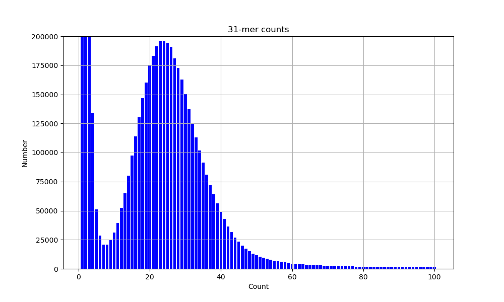
If you need help plotting, the python code for this can be expanded below.
Plotting code
import matplotlib.pyplot as plt

# Histogram data
data = [
    (2, 15484361),
    (4, 489010),
    (6, 94724),
    (8, 44768),
    (10, 49707),
    (12, 70508),
    (14, 98919),
    (16, 134835),
    (18, 179460),
    (20, 218909),
    (22, 254678),
    (24, 283570),
    (26, 306604),
    (28, 311785),
    (30, 307007),
    (32, 287181),
    (34, 267382),
    (36, 237045),
    (38, 206375),
    (40, 177546),
    (42, 146763),
    (44, 121426),
    (46, 99932),
    (48, 79153),
    (50, 62170),
    (52, 49436),
    (54, 39272),
    (56, 31315),
    (58, 25672),
    (60, 20977),
    (62, 16362),
    (64, 13319),
    (66, 11578),
    (68, 9804),
    (70, 8140),
    (72, 7398),
    (74, 6501),
    (76, 5969),
    (78, 5420),
    (80, 5036),
    (82, 4370),
    (84, 3992),
    (86, 4143),
    (88, 3854),
    (90, 3898),
    (92, 3799),
    (94, 3424),
    (96, 3135),
    (98, 2923)
]

x_values, y_values = zip(*data)

plt.figure(figsize=(10, 6))
plt.bar(x_values, y_values, color='blue')
plt.title('31-mer counts')
plt.xlabel('K-mer count')
plt.ylabel('Count')
plt.ylim(0, 200000)
plt.grid(True)
plt.show()
Exercise 3 Time the main loop which counts the k-mers and separately time
the loop which prints them out. Then, change the BTreeMap to a HashMap. How do
the times change? Change the HashMap to the implementation from use hashbrown::HashMap;
instead of the std crate. How do the times change now?
Optimising the code
This is relatively computationally intensive. How can we do better? Firstly, if we use the code above to encode the k-mers as 64-bit integers, our dictionary will be able to access the elements much faster as hashing the computer's word size is a lot faster than a string of unknown length. Secondly, rather than taking a slice from the sequence each time we could instead try to 'roll' the k-mer through the read, as to get to the next k-mer we just need to remove the first base removed and add a new last base.
Change your code as follows:
pub fn encode_base(base: u8) -> u8 {
    (base >> 1) & 0x3
}

pub fn rc_base(base: u8) -> u8 {
    base ^ 2
}

fn main() {
    let mut kmer_counts: HashMap<u64, usize> = HashMap::new();
    let k = 31;
    let mask = (1 << (k * 2)) - 1;
    let filenames = vec!["ERR8158023_1.fastq.gz", "ERR8158023_2.fastq.gz"];
    for filename in filenames {
        eprintln!("Parsing: {filename}");
        let mut reader =
            parse_fastx_file(filename).unwrap_or_else(|_| panic!("Invalid path/file: {filename}"));
        while let Some(record) = reader.next() {
            let seqrec = record.expect("Invalid FASTA/Q record");
            let mut fwd_kmer: u64 = 0;
            let mut rev_kmer: u64 = 0;
            for (idx, base) in seqrec.seq().iter().enumerate() {
                let fwd_base = encode_base(*base);
                let rev_base = rc_base(fwd_base);
                fwd_kmer <<= 2;
                fwd_kmer |= fwd_base as u64;
                fwd_kmer &= mask;
                rev_kmer >>= 2;
                rev_kmer |= (rev_base as u64) << ((k - 1) * 2);
                rev_kmer &= mask;
                // Once the first valid k-mer has been filled
                if idx >= k {
                    let key = if fwd_kmer < rev_kmer {fwd_kmer} else {rev_kmer};
                    *kmer_counts.entry(key).or_insert(0) += 1;
                }
            }
        }
    }
    // TODO: Counting and hist code go here
}
This uses some of the bitshifting tricks we used in the first session.
Add your count code at the end. How long does the code take to run now?
Other data structures
Another data structure, beyond the scope of this introduction, is the
Bloom filter
which can determine whether an item is present in a set, but with a false positive
rate. If you would like to try this, there is an implementation in the bloom
crate.
Further thoughts and reading
Try profiling your code with flamegraph. What takes the longest? Reading the file, processing the sequence, or adding to the dictionary?
If you want to understand more about why the k-mer counting takes a long time you can read about the CPU cache in the algorithmica book, but be warned it is quite involved! A perhaps more lively demonstration of this issue is in this computerphile video.
A blocked-bloom filter is a more cache-efficient implementation. Using this as the first stage to filter singleton k-mers, followed by a dictionary for counting gives an error-free k-mer count that is around twice as slow as the best implementations. Parallelism can be used to improve this further.
For all of these dictionary-based implementations the complexity overall is
linear with the number of k-mers in the file. So while the total speed changes
by a constant factor, all take twice as long to run with twice as many reads
in the input (try reading just one of the fastq files to confirm this). What
about the BTreeMap?
Object oriented Programming
In this section we'll use structure our code as objects. It may be a good idea
to first review the introduction to struct.
An object (used interchangeably here with struct and class) contains two things:
- Variables, also known as state.
- Methods, which can act on this state.
These are defined in the struct block and the impl block respectively. These are
defined for any instance of this class. Specific instances (variables) of the class,
where you use let variable: Class = Class::new() have specific values for each of their variables.
Variables should typically not be accessed directly, and instead use methods to read or write their values.
It is common to define a public (pub) new() method to create an instance of the class.
This may compute the state from some of the arguments. For example:
#[derive(Debug, Default)]
struct Cat {
    name: String,
    age: usize,
    tabby: bool,
}

impl Cat {
    pub fn new(name: &str, age: usize, pattern: &str) -> Self {
        let tabby = if pattern == "stripes" {true} else {false};
        Self {name: name.to_string(), age, tabby}
    }

    pub fn age(&self) -> usize {
        self.age
    }

    pub fn year_passed(&mut self) {
        self.age += 1;
    }

    pub fn is_tabby(&self) -> bool {
        self.tabby
    }
}

pub fn main() {
    let martha = Cat::new("Martha", 6, "stripes");
    let annie = Cat::new("Annie", 7, "tuxedo");
    println!("{:?} {:?}", martha, annie);
}
Methods usually take a reference to self
to allow access to the state, with mut if any of the state is changed.
The return type of new() should the the type of the class itself, i.e. Cat.
Using the keyword Self (note the capital) is the same in the above example of
writing Cat, but with the advantage that if the class name is ever changed this doesn't
have to be updated more than once.
Deriving Debug lets us print the contained values with the debug directive {:?},
deriving Default allows a default (empty) value of the class to be set.
You can also make a new class directly by defining all of its state:
#![allow(unused)]
fn main() {
struct Cat {
    name: String,
    age: usize,
    tabby: bool,
}

let martha = Cat {name: "Martha".to_string(), age: 6, tabby: true};
}
But it's usually better to define a new() method (sometimes known as the constructor)
so you have more control.
More advanced uses
We will not use these here, but the following are common in object-oriented programming.
You may sometimes also use inheritance, where objects have relationships like
parent and child sharing some of their variables and methods. An example
would be a parent class Animal with variables legs and method walk(), and child
classes Cat and Dog which inherit both of these and then add their own variables
(e.g. tabby and gundog) and methods meow() and bark(). These may be overriden,
for example the Cat class may provide its own definition of the walk() method.
Polymorphism is where a the actual function definition used is different depending
on the type used. This is very common in R code, where print() and plot()
and summary() all do different things depending on the type they are passed. Try
making a linear regression with model <- lm(y ~ x) and running these functions on model. If
you pass these functions a data.frame or a phylo object they will all still run,
but be running different functions.
A practical example: Gaussian blur
As our exercise, we will use rust to apply a Gaussian blur on a grayscale image. You can find a good overview of how to do this here: https://stackoverflow.com/a/1696200
We'll do this in four steps:
- Calculate the Gaussian filter
- Create a struct for 2D arrays (matrices)
- Apply the filter across the image (convolution)
- Putting it all together on a real image
Step 1: Calculating the Gaussian filter
Let's first create a function in main() which makes a Gaussian filter of a given size
radius:
use std::f64::consts::PI;

fn main() {
    let radius = 3;
    let sigma = max((radius as f64 / 2), 1.0);
    let kernel_width = (2 * radius) + 1;

    // We will add the code for this in step 2
    let kernel = PixelArray::zero_array(kernel_width, kernel_width);
    for x in -radius..radius {
        for y in -radius..radius {
            // Calculate the Gaussian density for given x, y
            let density = todo!()
            println!("{x} {y} {density}");
            // We will add the code for this in step 2
            kernel.set_pixel(x + radius, y + radius, density);
        }
    }
}
Add the code to calculate the Gaussian density at the given (x,y), using the following formula: \[ G(x, y) = \frac{1}{2\pi\sigma^2}\exp(-\frac{x^2 + y^2}{2\sigma^2}) \]
The value of sigma is set at the start, and the constant PI is already imported.
Step 2: Struct for 2D arrays
The pixels of our image and our filter are both going to be 2D arrays of numbers
which we'll want to be able to access given a pair of (x,y) co-ordinates.
We could use a vector of vectors Vec<Vec<i32>> which can be accessed by a[1][2],
but instead we'll take a more efficient approach of using a single vector
wrapped around rows (recall the row-major format in the first session):
#![allow(unused)]
fn main() {
struct PixelArray {
    pixels: Vec<f64>,
    height: usize,
    width: usize
}

impl PixelArray {
    fn get_pixel(&self, x: usize, y: usize) -> f64 {
        let index = x + y * self.width;
        self.pixels[index]
    }

    fn set_pixel() {
        todo!()
    }
}

}
Try and fill in the set_pixel() function definition to take an \(x\), \(y\) and value
which updates the given pixel. Then create a simple PixelArray, and try getting and
setting some pixel values. You can edit the above code directly, but it may be better
to start your own rust project by running cargo new.
What happens if you pick an \(x\) or \(y\) which is invalid? Modify the functions
to check for these cases and throw an error message using Option:
#![allow(unused)]
fn main() {
struct PixelArray {
    pixels: Vec<f64>,
    height: usize,
    width: usize
}

impl PixelArray {
    fn get_pixel(&self, x: usize, y: usize) -> Option<f64> {
        if x > self.width || y > self.height {
            None
        } else {
            let index = x + y * self.width;
            Some(self.pixels[index])
        }
    }
}
}
Do the same check for set_pixel(), but use panic!() to error in the function
if an invalid x or y is given.
Then, add an empty_array() function to the impl, which should create a PixelArray
full of zeros with the specified size:
#![allow(unused)]
fn main() {
fn zero_array(height: usize, width: usize) -> Self {
    let pixels = vec![0; height * width];
    Self { pixels, height, width }
}
}
Finally, add a function to the impl block which normalises the kernel, making all the values sum to 1.
Step 3: Apply the image across the filter (convolution)
We are now going to apply the blur, which we do using a convolution. For an image, this means running the kernel across the image, multiplying each overlapping pixel value by the corresponding entry in the kernel, and summing these to get the new value for that pixel. This averages across the kernel, with a density given by the Gaussian function.
Once done in the main block, after loading your image (in step 4) you'll sweep over all the pixels row-by-row as follows:
#![allow(unused)]
fn main() {
for y in 0..image.height {
    for x in 0..image.width {
        image.apply_kernel(x, y, &kernel);
    }
}
}
But first we need to define the convolution function apply_kernel(). Add this
as a method to PixelArray in the impl block as follows:
#![allow(unused)]
fn main() {
impl PixelArray {
    // get_pixel(), set_pixel() etc functions here...
    //...

    fn apply_kernel(&mut self, x_centre: usize, y_centre: usize, kernel: &PixelArray) -> f64{
        // NB: this prevents overflow at the edges, but the kernel is not normalised correctly
        let kernel_radius = (kernel.height - 1) / 2;
        let x_min = x_centre.saturating_sub(kernel_radius);
        let x_max = (x_centre + kernel_radius).min(self.width - 1);
        let y_min = y_centre.saturating_sub(kernel_radius);
        let y_max = (y_centre + kernel_radius).min(self.height - 1);

        let mut pixel_value = 0.0;
        for x in x_min..=x_max {
            for y in y_min..=y_max {
                let kernel_val = kernel.get_pixel(x + kernel_radius - x_centre, y + kernel_radius - y_centre);
                // Add to the pixel value by multiplying the pixel value at (x,y) by kernel_val
                todo!();
            }
        }
        pixel_value // return the result of the convolution at that pixel
    }
}
}
When you are using a usize, saturating_sub() will mean any subtraction which would be \( < 0\) will be truncated at zero
rather than causing an error. The first five lines therefore find the range of pixels
surrounding the centre pixel which don't overflow outside the boundary. (We are
ignoring that at the edges we are missing some of the kernel).
Complete this function in so that pixel_value is summed correct in the inner loop,
and at the end so that pixel_value is assigned to the correct pixel in the image
by calling .set_pixel().
Step 4: Putting it all together on a real image
Let's blur the following image, which for simplicity is in black and white:

This is a bitmap, which is just an array of pixels plus some metadata, almost identical to your PixelArray
struct. The values are u8 rather than f64, but are also stored in row-major order with a width and height.
Right click the image and save this into your rust project directory.
Rather than working out how to load and save bitmaps, we'll use the bmp package. To
use this add to your Cargo.toml:
[dependencies]
bmp = "*"
and add:
#![allow(unused)]
fn main() {
extern crate bmp;
use bmp::Pixel;
}
at the top of main.rs. Using packages is usually this easy, as cargo will deal with
downloading and compiling them for you. We'll go into a bit more detail at the end.
Using the package is easily and maps very well onto your existing struct. You can read
the package docs to work out how to load and save bitmaps, or just add the following
functions I made earlier to your impl (click the arrow to expand)
Loading and saving bitmaps
#![allow(unused)]
fn main() {
impl PixelArray {
    fn from_bitmap(file: &str) -> Self {
        let img = bmp::open(file).unwrap_or_else(|e| {
            panic!("Failed to open: {}", e);
         });
        let mut image_array = Self::empty_array(img.get_height() as usize, img.get_width() as usize);
        for y in 0..image_array.height {
            for x in 0..image_array.width {
                let px = img.get_pixel(x as u32, y as u32);
                let px_avg = px.b as f64; // Just take a single pixel, as r,g,b are all the same in a B&W image
                image_array.set_pixel(x, y, px_avg);
            }
        }
        image_array
    }

    fn to_bitmap(&self, file: &str) {
        let mut img = bmp::Image::new(self.width as u32, self.height as u32);
        for y in 0..self.height {
            for x in 0..self.width {
                let px_val = (self.get_pixel(x, y)) as u8;
                let px = Pixel::new(px_val, px_val, px_val); // Set r,g,b all the same for B&W
                img.set_pixel(x as u32, y as u32, px);
            }
        }
        img.save(file).unwrap_or_else(|e| {
            panic!("Failed to save: {}", e)
        });
    }
}
}
To get this all to work, add to your main() function after the kernel is set up:
- Load the tiger image using
PixelArray::from_bitmap("tiger.bmp") - Add the convolution loop in from above which calls
.apply_kernel()over every pixel. - Save the blurred image using the
.to_bitmap()function.
You can then run your program with cargo run. If it works, it should look like this:

Try with different radiuses of blur and see what happens.
Is there any difference in runtime between the debug and release versions?
Software engineering
Note: This chapter does not contain any practical material. Working through the tasks needed to make software is most rewarding with your own code, problem and potential users – it's a bit dry to practice all of this with contrived examples. Instead, here I give mostly subjective reflections and lessons I have learned about making academic software. I hope this is a useful discussion for both novices and researchers who already have developed many software packages.
Our definition, for research code, of software is that it is designed to be used by other people. Intention and thought has specifically been put into its use and reuse, usually both for end-users applying your method to new datasets, or for other developers who may wish to extend or maintain your code.
We will first discuss why you would want to do this at all, pitfalls and lessons in software engineering, and a summary of my top tips for doing this as part of your research career.
The module then lists the steps required to make your methods into software and some tools to help you achieve them.
Contents:
- Why bother?
- Lessons learned from my experiences
- Top tips
- Making a package – necessary steps
- Making a package – strongly recommended steps
- Making a package – good practice
Why bother?
It takes some time to make a piece of software, and even longer to support and maintain it. So why go through this?
The first advantages are practical. Having worked hard on your method, it's often only a small amount of extra initial work to make something that's more like a piece of software. Using this you can get a better and faster workflow, achieve better reproducibility, and increase the quality of your own results.
Once your software starts to get used by others, you'll see some advantages beyond your own work. It's a great basis for help people with less expertise in the field than you, and potentially starting collaborations. It increases the impact of your work, and makes the time you spent on the method more worthwhile.
Finally, for established software this can have a very positive impact on your own career. You can become quite famous (famous for a scientist anyway) through well-used and well-liked software.
Drawbacks
It's not all roses:
- It's hard to get funding for software development.
- It is not always a well-respected research activity, especially at early career stages.
- User issues can be frustrating.
- Software maintenance can last a lot longer than you originally planned.
For me, all of the above outweigh this – particularly the joy in helping others and the improved workflows in my own research.
So do consider if it's worth it for you overall, and whether it's worth it for the specific method or piece of code you are writing. Not everything should be a software package!
Lessons learned from my experiences
Here is a highly subjective list of lessons I think I have learnt along my way:
The basics:
- Make installation as easy as possible.
- The next most important thing after installation is documentation.
- Include tutorials with real data in the documentation.
- Actively seek feedback on your documentation.
- License your software.
- A good name (at least possible to say out loud) and logo are worth thinking about. Consider your audience a bit here. Bioinformaticians, yes a silly backronym or LOTR reference will go down well. Clinicians or public health? Maybe something more sensible.
- Choose the right language for the job (or multiple languages). Your favourite, good package or community support, learning something new are all good reasons to go for something. R is not better than python and python is not better than R.
- Add some testing, but not necessarily unit testing.
Maintaining software:
- Write down ideas or possible bugs as issues, with enough information to understand them in a year's time.
- When working with others use an organisation repo not your own one to get better control over access.
- Split your packages up into smaller pieces/sub-packages.
- Start to think about life-cycle. Retire old packages which are no longer worth your time to maintain. By this I mean freeze the code and do not make further changes or fixes.
- Write (and supervise writing of) maintainable code. Good luck with this one. Use an organisation repository
- Avoid dependencies if easy to do so.
- With later-stage software, prioritise fixing bugs over adding features.
- For bigger packages, unit tests are worthwhile.
Community interactions:
- Not everyone needs to use your approach. You might be convinced you have the best software, but people's needs are different and you can't make something that equally satisfies everyone.
- Users can be callous! They are interested in finding a method/software tool which is best for their needs. Don't expect if you sink a lot of time into helping someone that it will definitely be useful for their needs.
- Redirect email queries to github. Then everyone can see them and their solution, and other people can help answer them.
- Don’t solve every problem, it’s ok to say no. Think about how many people would benefit from a change.
- It’s ok to disagree with others on style (including this guide), be pragmatic and even if you feel inexperience in software engineering your opinion matters.
Top tips
- Make installation easy (should typically take around a day). This is the first hurdle. Not installable, not reusable.
- Make a sensible interface and defaults (typically around half a day). Think about what users typically want, and make it easy for them to get going.
- Make good documentation (at least 1-2 days). You will save yourself and others so much time by investing effort in making good documentation.
As with other sections of this course, I would advise to think about where to spend your time on software development. It's easy to fall into a hole of adding features, optimising code, perfecting the packaged, even if it might not be that useful. Be intentional with where you spend your time in software.
In my experience activities can roughly be split as follows:
High impact: installation, documentation, solving your own research questions.
Medium impact: basic tests, making it look good, interface design, speeding up frequently used code.
Low impact: issues affecting a single person, speeding up rarely used code, adding features
It’s also ok to do things that you enjoy – not every decision needs to be based on impact. Although I've spent most of this course saying the opposite, sometimes adding a feature or doing a better reimplementation can be very satisfying.
Making a package – necessary steps
Software engineering is a career in its own right and we can't hope to cover all that's involved here. But here's an attempt at the basic steps you need to take your research code, probably a script, into something that's usable by others.
For all of these steps it's much easier to follow an examples from elsewhere. Once you've done it for yourself, you'll find that it's common to reuse the same patterns and techniques for new packages.
First of all:
- Pick a good name that's not too long or that's impossible to actually say, and isn't already taken by another package in your field. In genomics, do not make packages with a permutations of the letters 'ACGT'.
- Put your code on github or gitlab, if it's not already there.
Structuring code as a package
Most languages have three basic elements needed on top of a script to make something distributable:
- A file with some metadata about the package, often version, dependencies, authors. In python
setup.py, in RDESCRIPTION, and in rustCargo.toml. - Put code into functions in a subfolder (python
package/__main__.py, rustsrc/main.rsorsrc/lib.rs). - Define the
main()function or entry points/exported functions. Make the main function point towards an interface which runs your existing functions.
A single file is hard to navigate, so it's usually a good idea to split your code over files with a common purpose. Functions can be shared across the package. Ideally functions should be relatively short so they can be tested as standalone units (given some input, does the function produce the expected output).
In python making a package structure means you have to install the package before running it, so you may find it convenient to have a 'runner' file in the top directory:
from mypackagename.__main__ import main

if __name__ == '__main__':
    main()
Make a sensible interface
Here by interface I mean a command line interface (CLI). Of course graphical interfaces or websites which run your code are possible and preferred by many users, but these are much more work and are beyond the current scope of this guide.
Running the program with the -h option should show information about the different
options and their defaults. Running with -v/--version/-V should give the version.
Writing code to parse argv (the actual text given on STDIN by the user) is very
tedious and you should use a package to do it for you:
- Python: argparse or docopt packages.
- R: roxygen2 and docstrings above exported function.
- Rust: clap package.
- C++ you can use Boost.Program_options, but a header-only library such as popl will be easier to support.
Try and make your commands simple (i.e. short), and run and work well with the chosen defaults for most users. Be cautious about adding too much or too little flexibility. The former makes getting started with the interface harder, the latter means that the code won't work for as many cases. If possible, getting user feedback can help guide you.
Although a good CLI will be somewhat self-documenting, giving examples, and putting these in the README or main documentation is a good idea. Make sure they run by running them yourself. What about when your code changes, will you remember to check they still run? We'll talk about this in tests and continuous integration below.
If you have a more complex package that performs multiple tasks, consider making subcommands
for each of these. A classic example is git, which has subcommands such as git merge, git commit, git push etc, each
with their own help. docopt and clap have good support for this.
Here's an example from one of my packages which uses clap. Running the program
gives an overview of all its different functions.
Split k-mer analysis

Usage: ska [OPTIONS] <COMMAND>

Commands:
  build     Create a split-kmer file from input sequences
  align     Write an unordered alignment
  map       Write an ordered alignment using a reference sequence
  distance  Calculate SNP distances and k-mer mismatches
  merge     Combine multiple split k-mer files
  delete    Remove samples from a split k-mer file
  weed      Remove k-mers from a split k-mer file
  nk        Get the number of k-mers in a split k-mer file, and other information
  cov       Estimate a coverage cutoff using a k-mer count profile (FASTQ only)
  help      Print this message or the help of the given subcommand(s)

Options:
  -v, --verbose  Show progress messages
  -h, --help     Print help
  -V, --version  Print version
Running a subcommand with -h gives more details:
Create a split-kmer file from input sequences

Usage: ska build [OPTIONS] -o <OUTPUT> <SEQ_FILES|-f <FILE_LIST>>

Arguments:
  [SEQ_FILES]...  List of input FASTA files

Options:
  -f <FILE_LIST>                   File listing input files (tab separated name, sequences)
  -o <OUTPUT>                      Output prefix
  -k <K>                           K-mer size [default: 17]
      --single-strand              Ignore reverse complement (all contigs are oriented along same strand)
      --min-count <MIN_COUNT>      Minimum k-mer count (with reads) [default: 5]
      --min-qual <MIN_QUAL>        Minimum k-mer quality (with reads) [default: 20]
      --qual-filter <QUAL_FILTER>  Quality filtering criteria (with reads) [default: strict] [possible values: no-filter, middle, strict]
      --threads <THREADS>          Number of CPU threads [default: 1]
  -v, --verbose                    Show progress messages
  -h, --help                       Print help (see more with '--help')
  -V, --version                    Print version
Add a README
Github will very insistent that you add a README. There seem to be two main types. Both start with a title and basic description of what the package does.
The first type, and probably what you should start off with, is to document installation and usage, adding all of your documentation to it as you go. Here's an example:
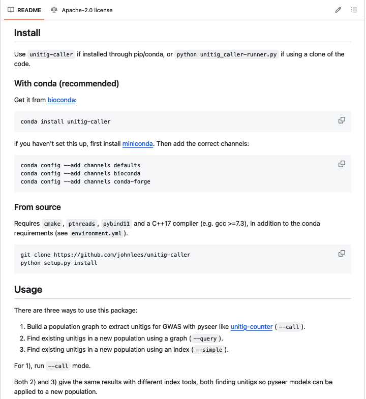
As the resources around the package increase, the README often just points to other resources in a structured manner, and offers some reassuring badges that suggest lots of testing is being run. Here's an example:

Pick and add a license
You'll also want to add a LICENSE file to tell others how your code can and can't be
used and reused. Sometimes you'll also want a separate NOTICE file which has your
name – some licenses end with a section to be modified which goes in this file,
see this example:
There are three basic types of license:
- Copyleft e.g. GPLv3, APGLv3. These mandate that if your code is reused the package which reuses it must use the same license, which precludes its use in most commercial/closed source settings.
- Permissive e.g. Apache-2.0, BSD-3, MIT or the Unlicense. Your code can be reused for any purpose, as long as you are given credit (the Unlicense waives this too).
- Copyright. Others cannot reuse your code without your explicit permission (and possibly payment). This is the default without a license, or if you want to retain rights by licensing through your organisation.
Note, a license is different from being open or closed source (which is not shared publicly at all). Typically the differences in licenses focus on reusing the code you have developed in other projects. Licenses also state that you have no liability and make no promises if the code doesn't work.
Check your organisation's advice or see https://choosealicense.com. In my opinion using a permissive license is usually best.
Tag a release
It's very useful in papers and for reproducibility for users (including yourself) to be able to state which version of the code they used. Once you start getting issues knowing the version used is invaluable.
On git, tags are a convenient name for a specific commit. Like commits, they can be made on your clone and pushed to the remote (i.e. github).
You'll want to use semantic versioning: v1.0.0 (MAJOR.MINOR.PATCH):
- MAJOR version when you make incompatible API changes i.e. old commands, files etc stop working with this version.
- MINOR version when you add functionality, but in a backward compatible manner.
- PATCH version when you make backward compatible bug fixes
Start with v0.1.0 and increment from there. Before v1.0.0 you make no promises that there won't be breaking changes, so usually wait until you're sure everything has settled down before releasing it! (often many years).
Releases can be made on github on the sidebar, adding notes about what has changed
and potentially executables. It will ask for a 'release name' for which mypackagename v0.1.0
is a good choice. If you haven't made a tag, this can automatically create one for you.
Making a package – strongly recommended steps
These two steps are not strictly necessary to make a software package, but I cannot emphasise enough how much of a difference they will make to its success as software. You should consider both as necessary, and that your return on investment in them will be very good (a stitch in time saves nine).
Add documentation
You really must tell people how to use the package, and what to expect when using it. I'm sure we've all been frustrating trying to use undocumented or poorly documented code.
Firstly, note that it’s for you as much as anyone else! I am likely the biggest user of my packages, and constantly use the documentation as a reference. Spending a couple of days, or even longer, writing everything down while it's fresh will save you time later. It will save even more time when you don't have to answer the same requests repeatedly.
Writing documentation is a bit of an art, and actively seeking feedback from users about what they like, what they find confusing and what they would like to see added. Unfortunately you won't hear from most people that tried your package and it didn't quite work for them.
A good starting place is the divio system:

This defines four types of documentation:
- How-to guides, which is usually your usage.
- Tutorials, which show a full worked example with some real or simplified data.
- Explanation, which in research code is most often taken from or expanding what's in the paper.
- Reference. API documentation in e.g. docstrings that explain individual functions. This is mostly for yourself, or others that might contribute to the code.
Don't forget to include commands, images and plots to make it more readable!
To actually make the documentation, it's a good idea just to include it as part of the code rather than making a separate document or website. It will then build every time you make the code and hopefully stay up to date. Just like in your README you can use Markdown to do most of your formatting in text, rather than needing to develop stylesheets. You can use:
sphinxin python. The default is to use reStructuredText rather than Markdown which has slightly more features, but you can change this.roxygen2in R.cargo docin rust.
Here is an example using sphinx:
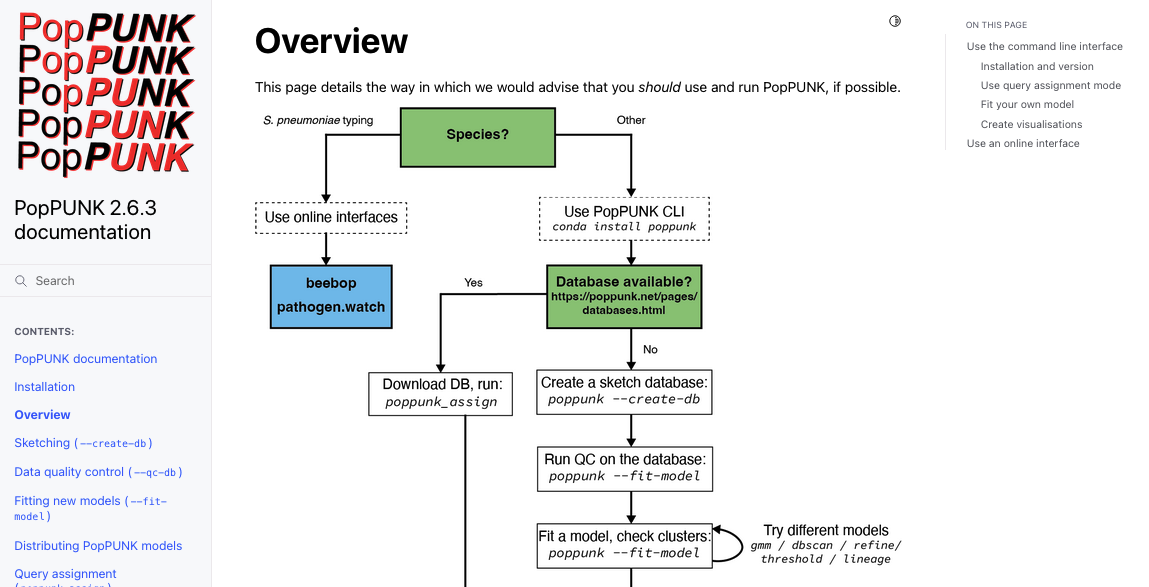
An example in R using roxygen:

Here is an example using rust:
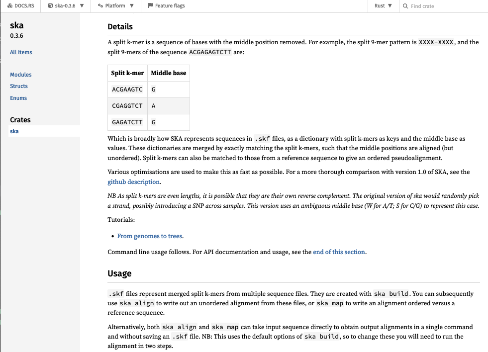
For all of these, you can see the code that generated the docs on github.
Good documentation
- Shows common failure modes and how to fix them.
- Shows figures and plots that are output, or which you have made externally.
- Gives examples of commands which can be run.
- Contains tutorials/vignettes which run through an analysis from end-to-end.
- Stays up to date and will run on the current version of the code.
Bad documentation
The worst type of documentation is documentation that doesn't exist. But these things can be a bit frustrating too:
- Some main function or options are completely undocumented.
- Gives error messages with no detail (e.g. ‘parsing failed’).
- Has out of date/unrunnable options.
Hosting your docs
Once you've built documentation by running one of the above options on your code, you can use the following free services:
- readthedocs.org (though this is becoming increasingly fiddly).
- github.io. Just make a branch that points to the html files.
- netlify supports many builders which integrate with github. You will however want a custom domain so you don't get a nonsense URL, which you will need to pay for (a tiny research cost honestly).
- Azure static websites similar to netlify, but currently still free for private organisation repos.
In rust, documentation will magically appear on https://docs.rs/ when you upload a crate.
Add installation methods
You should have at least one way to install your software, but having two different methods is a good starting aim as it's not uncommon for people to be unable to use one of them. Having more options isn't a bad idea, but probably has diminishing returns.
The fundamentals for each language are:
- For python you need to write a
setup.pyfile which you can then use withpip installto install your package. A more modern solution ispoetry. - For R using RStudio's 'New project' will get you started, then
devtools::install(). - For rust, just run
cargo install.
Assume that people do not have admin rights, so using sudo or similar is not going to work.
To depend or not to depend
Usually installing your software isn't too hard (especially if its an interpreted language), but any dependencies you've used are what starts to make things tricky. You shouldn't typically expect users to be able to install dependencies themselves, so using some form of package manager with dependency management is a must.
Here's a depressingly common scenario:
- Your package depends on
scikit-learnand works nicely with the current release. - Down the line the API changes and your function suddenly stops working with the current version, or worse has been removed entirely.
- At this point your software breaks.
- Unable or unwilling to fix this problem you didn't cause, you pin the version of
scikit-learnto be lower than or exactly the one which works. - Your other dependencies update to the new API.
- The package manager can no longer find a set of versions which satisfy the constraints.
So without maintenance everything stops working over time 😪.
You could just do everything from scratch and avoid dependencies entirely. In some areas, such as fundamental sequence analysis, this is a possibility. But using dependencies not only makes things quicker to develop, they are usually well-tested and more reliable and optimised than your own version could realistically be.
My advice is to take a pragmatic approach to each dependency. Could it easily be avoided? Then add it in yourself. Otherwise bite the bullet. Be slightly more avoidant of complex packages which require code to be compiled or use many languages (e.g. PyTorch) -- would a simpler solution avoid them? Sometimes that's a compromise you need to make with software, where 'it works for me' isn't good enough.
Also accept that pretty much everything needs at least some love and time to keep going. Is it worth it? Has it been superseded? At some point sunsetting your package and withdrawing active support can become the right option.
If this worries you:
- Make a docker container, see below (although this isn't entirely foolproof)
- Consider engaging with the software sustainability institute.
Official package repositories
Package repositories have the great advantage that they are very easy for users to work with as they have official support:
- Python – PyPI, submit with
twine upload. - R – CRAN or Bioconductor, submit with
devtools::release(). - Rust – https://crates.io, submit with
cargo publish.
Caveats:
- PyPI – dependencies don’t work properly in pip. You really can put anything on there.
- CRAN – difficult to pass all the checks.
All languages
The following methods should work for all languages and are a good addition to the official route:
- bioconda or conda-forge – user runs
conda install <package>which gives them a pre-built binary. compatible with their installed dependencies. Installs into an environment. - https://easybuild.io/ runs the build locally, which can give more efficient
- Docker and/or singularity – creates a snapshot of the whole environment which the user then pulls.
conda does resolve dependencies properly, but its use can cause difficulties for novices, especially with multiple environments. Creating recipes for your packages is quite easy, especially for python packages. Follow an example.
Docker/singularity are more effort to make and use, but have a (mostly) guaranteed environment and are a good backup when conda won't work. Note that docker typically requires admin rights to run, so having both is a good idea (use the converter). Make sure you give example commands of how to use the container, most users will not know what to do with a docker image.
Installing from source is good to include for your own reference, but not a route that most non-developer users will be able to follow, especially when dependencies are involved.
Making a package – good practice
Software engineers will probably do all of the following, but they are less critical (and more time-consuming) than the above points. Once you're used to them they can easily become part of every project, but starting out doing at least the basics here will help improve your code.
Add some tests
As researchers, we are typically pretty good at questioning results from code and usually come up with ways of diagnosing whether our output looks correct. Usually this means plotting the data.
In software engineering testing is a lot more formalised, usually by giving the program some input data and then mandating that it gives exactly the expected output. They are very useful with complex code for ensuring that when you change some code, it doesn't break anything elsewhere (known as a regression). Adding tests when you write new functionality also ensures that it actually works (and perhaps considers all the difficult edge cases).
There are three types of test that might be useful to add:
- Smoke tests which simply check you can install and run the package.
- Integration tests, which test a full command's workflow i.e. executing the whole program.
- Unit tests, which test the behaviour of a single function (unit).
Here is a smoke test in rust which tests the program can be run and it makes the output file:
#[test]
fn build_cli() {
    Command::new(cargo_bin("ska"))
        .current_dir(sandbox.get_wd())
        .arg("build")
        .arg("-f")
        .arg(rfile_name)
        .arg("-o")
        .arg("basic_build_opts")
        .args(&["-v", "--threads", "2", "-k", "31"])
        .assert()
        .success();

    assert_eq!(true, sandbox.file_exists("basic_build_opts.skf"));
}
Here is an integration test from the same file, which also tests the output is as expected:
#[test]
fn build_and_align() {
    let sandbox = TestSetup::setup();

    Command::new(cargo_bin("ska"))
        .current_dir(sandbox.get_wd())
        .arg("build")
        .arg("-o")
        .arg("basic_build")
        .arg("-k")
        .arg("15")
        .arg(sandbox.file_string("test_1.fa", TestDir::Input))
        .arg(sandbox.file_string("test_2.fa", TestDir::Input))
        .assert()
        .success();

    let fasta_align_out = Command::new(cargo_bin("ska"))
        .current_dir(sandbox.get_wd())
        .arg("align")
        .arg("basic_build.skf")
        .arg("-v")
        .output()
        .unwrap()
        .stdout;

    let correct_aln = HashSet::from([vec!['A', 'T'], vec!['C', 'T']]);
    assert_eq!(var_hash(&fasta_align_out), correct_aln);
}
Here is a unit test which tests a single function and the ways it can go wrong (the function and test are in the same file):
/// Adds a split k-mer which is a self-rc to the dict
/// This requires amibguity of middle_base + rc(middle_base) to be added
fn add_palindrome_to_dict(&mut self, kmer: IntT, base: u8) {
    self.split_kmers
        .entry(kmer)
        .and_modify(|b| {
            *b = match b {
                b'W' => {
                    if base == 0 || base == 2 {
                        b'W'
                    } else {
                        b'N'
                    }
                }
                b'S' => {
                    if base == 0 || base == 2 {
                        b'N'
                    } else {
                        b'S'
                    }
                }
                b'N' => b'N',
                _ => panic!("Palindrome middle base not W/S: {}", *b as char),
            }
        })
        .or_insert(match base {
            0 | 2 => b'W', // A or T
            1 | 3 => b'S', // C or G
            _ => panic!("Base encoding error: {}", base as char),
        });
}

#[cfg(test)]
mod tests {
    use super::*;

    #[test]
    fn test_add_palindrome_to_dict() {
        // Initialize the test object
        let mut test_obj = SkaDict::<u64>::default();

        // Test case 1: Updating existing entry
        test_obj.split_kmers.insert(123, b'W');
        test_obj.add_palindrome_to_dict(123, 1);
        assert_eq!(test_obj.split_kmers[&123], b'N');

        // Test case 2: Adding new entry with base 0
        test_obj.split_kmers.clear();
        test_obj.add_palindrome_to_dict(456, 0);
        assert_eq!(test_obj.split_kmers[&456], b'W');

        // Test case 3: Adding new entry with base 3
        test_obj.split_kmers.clear();
        test_obj.add_palindrome_to_dict(789, 3);
        assert_eq!(test_obj.split_kmers[&789], b'S');

        // Test case 4: Updating existing twice
        test_obj.split_kmers.insert(123, b'W');
        test_obj.add_palindrome_to_dict(123, 1);
        test_obj.add_palindrome_to_dict(123, 1);
        assert_eq!(test_obj.split_kmers[&123], b'N');
    }

    #[test]
    #[should_panic]
    fn test_panic_add_palindrome_to_dict() {
        // Test case 4: Panicking with invalid base
        let mut test_obj_panic = SkaDict::<u64>::default();
        test_obj_panic.add_palindrome_to_dict(987, 5);
    }

    #[test]
    #[should_panic]
    fn test_panic2_add_palindrome_to_dict() {
        // Test case 5: Panicking with invalid middle base
        let mut test_obj_panic = SkaDict::<u64>::default();
        test_obj_panic.split_kmers.clear();
        test_obj_panic.split_kmers.insert(555, b'A');
        test_obj_panic.add_palindrome_to_dict(555, 1);
    }
}
Integration tests are usually quite easy to write. However, with more complex code, if they fail you won't get information on what has failed and why. Many software engineers prefer to write unit tests to ensure errors are more precise, and furthermore believe that this writing code with testability in mind improves your coding practices.
Personally I would suggest a more relaxed approach to testing in research software, especially in your first forays into this area. Adding a smoke test and a couple of integration tests is a good way to get started.
As always, consider how much time it will take and whether you will benefit from it. More tests can also increase the burden on new contributors, so make sure they are checking functionality over style.
If you are writing unit tests I've found ChatGPT is good at writing them if you paste the function to be tested in. Note the style of unit testing requires that your code be written in testable units i.e. you need to write short functions with defined input and output, not giant functions with many different possible paths through them.
If you really want to go further in this direction you can also check your test coverage with codecov. This checks which lines of your code are actually being run when tested, to make sure that every possible path through the code has been checked. This is rarely necessary with research code, but if you add it and then make a small pull request with a new function, it can be useful to check you have actually tested your change.
Automate your tests using continuous integration (Github actions)
Much like documentation, tests are best when they are integrated as part of your code.
R and rust both have integrated tools to run the tests (devtools::check() and cargo test respectively),
for python you will probably want to use a package such as pytest and/or you can
write a wrapper script to run your tests.
It's hard to remember to do this with every change, and also make sure other contributors are checking the tests. Using continuous integration (CI), where an external server (usually virtual machine) automatically tries to install, run and test your code solves this.
Github actions will let you run code when you commit, create pull requests etc. Common examples are:
- Check tests pass (CI)
- Run a linter (see below)
- Make and upload a release (continuous deployment)
- Build the documentation
They are useful for anything you might forget to do! To set them up, you just
need to add YAML files in .github/workflows/. Check
out some examples to get started, and note that you can run almost any command you want.
People also like to put badges for their tests in the README, which I am sure you have
seen before:
![]()

![]()
![]()


Code quality
When we discussed this in the first iteration a question at the end was 'how can I keep getting better at coding?'. Two vague suggestions:
- Work with people (software engineers, research colleagues) who are have more experience than you, or your peers.
- Keep being interested in learning new patterns, check what recommended solutions in a language are.
Two concrete suggestions I will expand upon are code linting and code review.
Linting
Linters are programs which checks you code formatting and standard:
R CMD check- Python –
black - Rust –
cargo clippyandcargo fmt
These can give you really useful suggestions such as using a neater function, finding an unused or undefined variable. I prefer ones which will make sensible changes for you (better if you have tests to check everything still works). They can also be annoying! You certainly don’t have to follow it, and please don't get hung up on fixing every 'failure':
- CamelCase vs underscore_names
- Number of function args
- Spaces around arguments
- ‘complexity’
Implement code review
This is perhaps the best way to get better at coding. Asking someone to review all of your code in a package isn't viable, but updates, and small pieces of code are doable.
Here is a good workflow for making this work. Firstly, make contributions are small, clean, and usually to close a single issue. Then:
- Write your code on a branch
- Commit regularly
- Make sure tests are passing
- When ready, open a pull request
- Suggest a reviewer
- Reviewer comments, requests changes
- Make changes, make sure tests are passing
- Request re-review
- Reviewer merges PR into master/main branch
Who should review? You can ask other students, colleagues or your supervisor (if they are capable!). Anyone you would happily review for. It doesn't matter if they are more/less experienced than you.
How to review? Not like a paper! Make necessary changes, and add any helpful suggestions. Don't be pedantic. No comments are also fine, a lot of code is already good at the stage of a pull request.
Recursion and closures
This session covers two programming techniques which are very useful but I have found people often haven't come across or used in anger.
Recursion is when a function calls itself. This can really lend itself to neatly writing certain algorithms, and in those cases is often a lot simpler than an iterative algorithm.
Closures are functions which capture their environment. Often this means that there is a more general function which has some of its options bound to specific values, yielding a more specific function which is then called just with the unbound arguments. These work really neatly in languages such as R where variables can be functions.
Another similar topic I might add here would be generators, which are functions which
return but retain their internal state. In python this is easily done with the yield keyword. However these aren't implemented in many languages yet so I will
omit them here, but you may want to look them up.
This session will have a brief overview and example, followed by a more challenging example for you to try. Solutions are at the end, but try not to look at them until you've given it a go.
I am going to give examples in rust, but you can use python or R just as easily for this module.
Recursion
The golden rule of recursion: make sure there is an exit condition for the function
For some reason the example often used for recursion is calculating the Fibonacci function \( f(x) = f(x - 1) + f(x - 2) \):
#![allow(unused)]
fn main() {
pub fn fibonacci_recursive(x: i32) -> i32 {
    // Remember the '_' branch is 'else'
    match x {
        0 => 0,
        1 => 1,
        _ => fibonacci_recursive(x - 1) + fibonacci_recursive(x - 2)
    }
}

let fib: Vec<i32> = (0..10).map(|x| fibonacci_recursive(x)).collect();
println!("{fib:?}");
}
But this clearly wasteful as we evaluate the same values repeatedly. This is a good
place to note the cached library which
stores previous runs of the function with the same input parameters, and makes the
above code a lot more efficient:
use cached::proc_macro::cached;

#[cached]
pub fn fibonacci_recursive(x: i32) -> i32 {
    match x {
        0 => 0,
        1 => 1,
        _ => fibonacci_recursive(x - 1) + fibonacci_recursive(x - 2)
    }
}

let fib: Vec<i32> = (0..10).map(|x| fibonacci_recursive(x)).collect();
println!("{fib:?}");
Note there is a similar decorator available in python.
This function is probably more obviously done with an iterative function anyway:
#![allow(unused)]
fn main() {
pub fn fibonacci_iterative(x: i32) -> i32 {
    if x == 0 || x == 1 {
        return x
    } else {
        let (mut fib, mut fib_minusone, mut fib_minustwo) = (0, 0, 1);
        for _ in 1..=x {
            fib = fib_minusone + fib_minustwo;
            fib_minustwo = fib_minusone;
            fib_minusone = fib;
        }
        fib
    }
}

let fib: Vec<i32> = (0..10).map(|x| fibonacci_iterative(x)).collect();
println!("{fib:?}");
}
For something more complex to which recursion is well suited, let's try something we all fondly remember, the flood fill from MS paint.
Let's reuse our PixelArray image code from the data structures module:
#![allow(unused)]
fn main() {
use core::fmt;

extern crate bmp;
use bmp::Pixel;

struct PixelArray {
    pixels: Vec<f64>,
    height: usize,
    width: usize
}

impl PixelArray {
    fn get_pixel(&self, x: usize, y: usize) -> f64 {
        let index = self.get_index(x, y);
        self.pixels[index]
    }

    fn set_pixel(&mut self, x: usize, y: usize, value: f64) {
        let index = self.get_index(x, y);
        self.pixels[index] = value;
    }

    fn get_index(&self, x: usize, y: usize) -> usize {
        if !self.valid_index(x, y) {
            panic!("Invalid index!");
        }
        x + y * self.width
    }

    fn valid_index(&self, x: usize, y: usize) -> bool {
        x < self.width && y < self.height
    }

    fn from_bitmap(file: &str) -> Self {
        let img = bmp::open(file).unwrap_or_else(|e| {
            panic!("Failed to open: {}", e);
         });
        let mut image_array = Self::empty_array(img.get_height() as usize, img.get_width() as usize);
        for y in 0..image_array.height {
            for x in 0..image_array.width {
                let px = img.get_pixel(x as u32, y as u32);
                let px_avg = px.b as f64;
                image_array.set_pixel(x, y, px_avg);
            }
        }
        image_array
    }

    fn to_bitmap(&self, file: &str) {
        let mut img = bmp::Image::new(self.width as u32, self.height as u32);
        for y in 0..self.height {
            for x in 0..self.width {
                let px_val = (self.get_pixel(x, y)) as u8;
                let px = Pixel::new(px_val, px_val, px_val);
                img.set_pixel(x as u32, y as u32, px);
            }
        }
        img.save(file).unwrap_or_else(|e| {
            panic!("Failed to save: {}", e)
        });
    }
}
}
Consider this pre-prepared tiger:

Right click and save the bitmap to get your input image.
What we want to do is fill in all of the white pixels in the bounded region as black. One
way of doing this is to turn the pixel we click on, the start_pixel, black. Then we can check
its neighbours, filling them in as black if they are currently white, and not doing anything
if they are already black. Then, for each of the originally white pixels, we would check its neighbours
and do the same thing. As we don't know the start and end of the bounded regions it's hard to do this in
a loop. However, the function of checking white/black and recolouring, then doing the same on the neighbours
is quite easy. We just need to call the function again within itself. This is recursion.
So, have a look at flood_fill() function in the code below which shows how to put this
together to make a paint bucket function:
use std::collections::HashSet;

extern crate bmp;
use bmp::Pixel;

impl PixelArray {

    pub fn flood_fill(&mut self, start: (usize, usize), filled: &mut HashSet<(usize, usize)>) {
        filled.insert(start); // Keep track of nodes already processed
        // Change this pixel from white to black
        if self.get_pixel(start.0, start.1) == 255.0 {
            self.set_pixel(start.0, start.1, 0.0);

            // Fill from left pixel outward
            let pixel_left = (start.0.wrapping_sub(1), start.1);
            if self.valid_index(pixel_left.0, pixel_left.1) && !filled.contains(&pixel_left) {
                self.flood_fill(pixel_left, filled);
            }
            // Fill from right pixel outward
            let pixel_right = (start.0.wrapping_add(1), start.1);
            if self.valid_index(pixel_right.0, pixel_right.1) && !filled.contains(&pixel_right) {
                self.flood_fill(pixel_right, filled);
            }
            // Fill from top pixel outward
            let pixel_top = (start.0, start.1.wrapping_add(1));
            if self.valid_index(pixel_top.0, pixel_top.1) && !filled.contains(&pixel_top) {
                self.flood_fill(pixel_top, filled);
            }
            // Fill from bottom pixel outward
            let pixel_bottom = (start.0, start.1.wrapping_sub(1));
            if self.valid_index(pixel_bottom.0, pixel_bottom.1) && !filled.contains(&pixel_bottom) {
                self.flood_fill(pixel_bottom, filled);
            }
        }
    }
}

fn main() {
    // Load the image
    let mut image = PixelArray::from_bitmap("tiger_lines.bmp");

    // let start_pixel = (239, 179); // does a stripe
    let start_pixel = (221, 173); // does most of the tiger
    let mut filled = HashSet::new();
    image.flood_fill(start_pixel, &mut filled);

    // Save the filled image
    image.to_bitmap("tiger_fill.bmp");
}
You should get something like this:

Try varying the start position.
Merge sort
Here is a more challenging problem to try, implementing a merge sort using a recursive algorithm. A merge sort works well when lists are nearly sorted. The idea is that we will take an unsorted list, split it into smaller lists, sort those smaller lists, then merge these sorted lists back together in order.
First, we need a merge function that will combine two sorted lists. We can do this by keeping two pointers (or iterators, in rust) which move down the lists. We take the currently smallest of the two, and move the pointer forward one in its list. This only goes through the lists once so is linear time.
#![allow(unused)]
fn main() {
pub fn merge(list1: &[i32], list2: &[i32]) -> Vec<i32> {
    let out_len = list1.len() + list2.len();
    let mut list_out = Vec::with_capacity(out_len);
    let mut list1_iter = list1.iter();
    let mut list2_iter = list2.iter();
    let mut list1_item = list1_iter.next().unwrap();
    let mut list2_item = list2_iter.next().unwrap();
    while list_out.len() < out_len {
        if list1_item < list2_item {
            list_out.push(*list1_item);
            list1_item = list1_iter.next().unwrap_or(&i32::MAX);
        } else {
            list_out.push(*list2_item);
            list2_item = list2_iter.next().unwrap_or(&i32::MAX);
        }
    }
    list_out
}
}
First, use assert!() to test this works with some simple input.
Then, try and write a recursive function to take two lists and sort them.
A handy function in rust is let (left, right) = list.split_at(index);. If you keep halving
the left and right lists, sorting them, then merging them in order (using the function above)
you'll get a sorted list. Also note that if you call merge() on two lists both of length 1, they
will be sorted (as a list of length 1 is already sorted by definition).
Some of the rust borrowing rules can be a bit of a headache here so if you are finding them annoying switch to python or R, the code will be very similar.
The golden rule of recursion: make sure there is an exit condition for the function
A solution can be found at the end.
Closures
Closures capture some of the environment when they are defined. They are really useful when you need to match a function's arguments. Typically this will be a function where you can't change the arguments, usually from an external library.
Here are some examples of doing this in python, rust and R.
python
Use the partial function from the functools library:
from functools import partial

def linear_regression_predict(x, slope, intercept):
    return intercept + x * slope

model1 = partial(linear_regression_predict, slope=-2, intercept=3)
predict_values = [-1, 0, 1, 5]
model1_predictions = [model1(x) for x in predict_values]
# [5, 3, 1, -7]
Here we have a more general function which predicts the y-axis value for a linear regression, given an input x value, slope and intercept. If we have fitted the slope and intercept we can 'bind' or 'capture' these to make a more specific predict function for that model. This is then more convenient to use elsewhere.
rust
The same example in rust:
pub fn linear_regression_predict(x: f64, slope: f64, intercept: f64) -> f64 {
    intercept + x * slope
}

pub fn main() {
    let slope = -2.0;
    let intercept = 3.0;
    let model1 = |x: f64| -> f64 { linear_regression_predict(x, slope, intercept) };
    let predict_values = vec![-1.0, 0.0, 1.0, 5.0];
    let model1_predictions: Vec<f64> = predict_values.iter().map(|x| model1(*x)).collect();
    println!("{model1_predictions:?}");
    // [5, 3, 1, -7]
}
Here you use || to define the input variables for the new function. Adding the move keyword
before this means the function will additionally take ownership of the other captured variables.
Note also the syntax for .map() also uses a closure. Closures can be used anywhere you want
to define a unnamed function, which is useful for very short functions. These are sometimes
called lambdas. We could use this to replace the linear_regression_predict() function entirely,
making the code more concise:
pub fn main() {
    let slope = -2.0;
    let intercept = 3.0;
    let predict_values = vec![-1.0, 0.0, 1.0, 5.0];
    let model1_predictions: Vec<f64> = predict_values.iter().map(|x| intercept + x * slope).collect();
    println!("{model1_predictions:?}");
    // [5, 3, 1, -7]
}
R
R has really great support for closures, as variables can be set to functions with no extra work:
linear_regression_predict <- function(x, slope, intercept) {
    intercept + x * slope
}

slope <- -2.0
intercept <- 3.0
model1 <- function(x) {linear_regression_predict(x, slope, intercept)}
predict_values <- c(-1.0, 0.0, 1.0, 5.0)
model1_predictions <- sapply(predict_values, model1)
model1_predictions
}
We can use sapply() in this way as the function operates on the value in the list.
Otherwise we would have to change the arguments to take a vector and give slope and intercept with every call.
Alternatively we could use apply() which has a ... argument allowing other parameters to be passed,
but with any other nesting of functions this gets complicated.
Optimiser using a closure
Let's stick with R and use a closure to make running an optimiser possible. A common example is Rosenbrock's function: \[f(x,y) = (a-x)^2 + b(y-x^2)^2 \]
As an R function:
rosenbrock <- function(a, b, x, y) {
    (a-x)^2 + b*(y-x^2)^2
}
The optim() function can be used to maximise or minimise a function, but the first
argument par needs to be a vector of parameters, which doesn't match the four defined
by that function.
Write a closure around rosenbrock() which captures a = 1, b = 100 and uses
x = input[1], y = input[2] so it can be passed to optim(). By default optim()
finds the minimum -- what is it, and at which co-ordinates?
If you are feeling brave, also define the derivative (for any \( a \) and \( b \)), and try some different optimisers.
Solutions are at the end.
Solutions
Merge sort
Merge sort:
pub fn merge(list1: &[i32], list2: &[i32]) -> Vec<i32> {
    let out_len = list1.len() + list2.len();
    let mut list_out = Vec::with_capacity(out_len);
    let mut list1_iter = list1.iter();
    let mut list2_iter = list2.iter();
    let mut list1_item = list1_iter.next().unwrap();
    let mut list2_item = list2_iter.next().unwrap();
    while list_out.len() < out_len {
        if list1_item < list2_item {
            list_out.push(*list1_item);
            list1_item = list1_iter.next().unwrap_or(&i32::MAX);
        } else {
            list_out.push(*list2_item);
            list2_item = list2_iter.next().unwrap_or(&i32::MAX);
        }
    }
    list_out
}

pub fn merge_sort(list: Vec<i32>) -> Vec<i32> {
    let (left, right) = list.split_at(list.len() / 2);
    let mut left = left.to_vec();
    let mut right = right.to_vec();
    if left.len() > 1 {
        left = merge_sort(left);
    }
    if right.len() > 1 {
        right = merge_sort(right);
    }
    merge(&left, &right)
}

fn main() {
    let mut list = vec![1,5,4,2,3,3,22,1,1];
    list = merge_sort(list);
    println!("{list:?}");
}
Optimiser
start_value <- c(-1.2, 1)

rosenbrock <- function(a, b, x, y) {
    (a-x)^2 + b*(y-x^2)^2
}
rosen <- function(x) {rosenbrock(1, 100, x[1], x[2])} # or we could write a <- 1; b <- 100 above
optim(start_value, rosen)

# With the gradient
gradient <- function(a, b, x, y) {
    ddx <- -2*a + 4*b*x^3 - 4*b*x*y + 2*x
    ddy <- 2*b*(y-x^2)
    c(ddx, ddy)
}
rosen_g <- function(x) {gradient(1, 100, x[1], x[2])}
optim(start_value, rosen, rosen_g, method = "BFGS", control = list(trace = 1))
Parallel programming
Contents:
- Introduction and theory
- Parallelising a for loop
- Using
rayonand iterables to make this much easier - Which work to parallelise?
This chapter covers the fundamentals in parallelism and implementation in rust. Subsections are then available covering examples in python, R and more complex examples in rust.
Using multiple CPU cores is a very common optimisation strategy. Modern laptops have 4-10 cores, and HPC nodes usually have 32. These give the best case speedups, though often efficiency \(\frac{t_{\mathrm{serial}}}{t_{\mathrm{parallel}} \times N_{\mathrm{CPUs}}}\) is less than 100% due to overheads of setting up parallelisation, such as spawning threads.
Introduction and theory
Some analysis does not require any use of shared memory or communication between threads. For example running the same program such as a genome assembler on 1000 different samples can be run as 1000 totally separate processes, and is probably best done as a job array or a pipeline like snakemake. These are known as 'embarrassingly parallel' tasks. You can also multithread embarrassingly parallel tasks when you are writing software, as it will be easier for many users to take advantage of.
What are good candidates for multithreading within a process? Usually where you have a part of your code that is particularly computationally intensive (usually as identified by some profiling) and uses the same variables/objects and therefore shared memory as the rest of the process.
When is it less likely to work? If multiple threads might write to the same variable or use the same resource then this makes things more complicated and often slower (but you can use atomic operations or mutexes to make this work). Additionally, making new threads usually has an overhead i.e. time cost, so the process being parallelised usually needs to run for a reasonable amount of time (at least greater than the cost of starting a new thread).
A common structure in code that can be parallelised is a for loop where each
iteration takes a non-negligible amount of time, as long as the loops do not
depend on each other. Where the results need combining, a common approach is
'map-reduce' which applies a function to multiple data using map then applies
a reduction function which combines the results from each of these processes.
A useful concept when planning how to parallelise your code is 'work', which is roughly the total amount of CPU time that needs to be spent on running the code, and whether and how this can be subdivided between independent parallel tasks. Ideally you want to split this work equally between the available CPU cores, as we always have to wait until the last core is finished to be done, then if one has more work it will make the whole process take longer.
Multiprocessing vs multithreading
Parallelism is often closely linked to the concept of asynchronous ('async') programming. Usually each line of code you write will have to finish running, and the result be available, before the next line is run. However there are many cases with I/O where it is useful for the process to continue running the rest of the code, and at some point later check if the async line has finished and collect its result (sometimes known as futures/promises):
- Waiting for user input.
- A webpage running some processing.
- Waiting for a query to a server to return.
- Waiting for a filesystem resource to be available, or finished being written to.
In terminal code making these kind of expected waits async allows code to be more efficient, as the main process can keep going and keep the CPU busy rather than idling waiting for an external resource. Underlying this idea, operating systems supports multiple threads, which it can switch in and out of the available CPUs to try and keep them busy (this is how you can run many applications at once, even on a single core CPU). On the web this is critical, as slow communication across the network is common, and webpages would completely freeze all the time if this wasn't done asynchronously.
With parallel code you are usually taking advantage of this system and launching
multiple threads which then (hopefully) get assigned to different cores and are
executed concurrently. This distinction isn't always that important, but does explain
why you often see other async tools together with concurrency options. Note that in python
threading is for async I/O and will
not make your CPU-bound code faster, whereas multiprocessing will.
Parallelising a for loop
Let's consider an example of finding whether numbers are prime:
#![allow(unused)]
fn main() {
fn is_prime(n: u32) -> bool {
    for div in 2..n {
        if n % div == 0 {
            return false;
        }
    }
    true
}

println!("2: {} 3: {} 4: {}", is_prime(2), is_prime(3), is_prime(4));
}
This starts from a very simple way to check if a number is prime: for every integer lower
than the input (excluding 1), check whether it divides exactly. We can do this with the
modulo function %, also known as the remainder.
We can do a simple optimisation by noticing that potential divisors > n/2 will never divide exactly, and furthermore that some of these will have already been checked by dividing by 2, 3, 4 etc. These conditions meet at the square root on the input:
#![allow(unused)]
fn main() {
fn is_prime(int: u32) -> bool {
    let upper = (int as f64).sqrt().floor() as u32;
    for div in 2..=upper {
        if int % div == 0 {
            return false;
        }
    }
    true
}

println!("2: {} 3: {} 4: {}", is_prime(2), is_prime(3), is_prime(4));
}
A further optimisation would be to only try dividing by primes as e.g. anything divisible by 6 will also be divisible by its prime factors 2 and 3. But as this involves keeping track of a list it's a bit more complex, so we'll go with the above.
Writing a function to find whether numbers are prime, including some timing, might look like this:
use std::time::Instant;

fn is_prime(int: u32) -> bool {
    let upper = (int as f64).sqrt().floor() as u32;
    for div in 2..=upper {
        if int % div == 0 {
            return false;
        }
    }
    true
}
fn main() {
    let size = 20000;

    let start = Instant::now();
    let mut primes = Vec::with_capacity(size - 1);
    for i in 2..size {
        primes.push((i, is_prime(i as u32)));
    }

    // Timing
    let end = Instant::now();
    let serial_time = end.duration_since(start).as_micros();
    println!("Serial done in {}us", serial_time);

    // Check results look ok
    println!("{:?}", &primes[0..10]);
}
The std::thread library gives us two tools for parallelisation:
::spawnwhich asynchronously runs the contained function in a new thread. The operating system should be able to run this thread on a different CPU core.::joinwhich waits for a spawned thread to finish, and gets the return value as a result.
So, we could try and parallelise this by spawning a new thread for every iteration of the loop, so that each integer's computation occurs on a new thread, which can potentially run in parallel:
use std::time::Instant;
use std::thread;

fn is_prime(int: u32) -> bool {
    let upper = (int as f64).sqrt().floor() as u32;
    for div in 2..=upper {
        if int % div == 0 {
            return false;
        }
    }
    true
}
fn main() {
    let size = 20000;

    let start = Instant::now();
    let mut primes = Vec::with_capacity(size - 1);
    let mut threads = Vec::with_capacity(size - 1);

    // Spawn the threads
    for i in 2..size {
        let thread_join_handle = thread::spawn(move || {
            is_prime(i as u32)
        });
        threads.push(thread_join_handle);
    }

    // Collect the results with join
    for (i, thread) in threads.into_iter().enumerate() {
        let result = thread.join().unwrap(); // join returns a result, which should be `Ok` so we can safely unwrap it
        primes.push((i + 2, result));
    }

    // Timing
    let end = Instant::now();
    let parallel_time = end.duration_since(start).as_micros();
    println!("Parallel done in {}us", serial_time);

    // Check results look ok
    println!("{:?}", &primes[0..10]);
}
But this is much slower than the serial version! On my laptop, this takes >2500x longer. This is due to the overhead of spawning 20k threads, which in most cases take longer than the actual computation they contain.
One solution would be to divide the total work into more equal sized chunks, and only spawn the threads once for each core we want to use:
use std::time::Instant;
use std::thread;

fn is_prime(int: u32) -> bool {
    let upper = (int as f64).sqrt().floor() as u32;
    for div in 2..=upper {
        if int % div == 0 {
            return false;
        }
    }
    true
}
fn main() {
    let size = 20000;

    let start_p = Instant::now();

    // Split the work
    let threads = 4;
    let mut work = Vec::new();
    for thread in 0..threads {
        let work_list: Vec<u32> = ((2 + thread)..size).step_by(threads).map(|x| x as u32).collect();
        work.push(work_list);
    }

    // Spawn the threads on each chunk of work
    let mut thread_results = Vec::new();
    for i in 0..threads {
        let work_for_thread = work[i].clone(); // This copy is needed, or we can use `sync::Arc` to avoid it
        let thread_join_handle = thread::spawn(move || {
            let mut work_results = Vec::new();
            for j in work_for_thread {
                work_results.push((j, is_prime(j as u32)));
            }
            work_results
        });
        thread_results.push(thread_join_handle);
    }

    // Collect the results with join
    let mut primes = Vec::new();
    for thread in thread_results {
        let mut result = thread.join().unwrap();
        primes.append(&mut result);
    }

    // Timing
    let end_p = Instant::now();
    let parallel_time = end_p.duration_since(start_p).as_micros();
    println!("Work splitting done in {}us", parallel_time);

    // Check results look ok
    println!("{:?}", &primes[0..10]);
}
This gives me a speedup of about 1.5x using the four threads. As I increase the size, this gets more efficient.
When you are profiling the time taken make sure you don't include the compile time, and include optimisations. The best way is to run cargo build --release first. Then run target/release/<name>.
Adding time before your command is also helpful for seeing if multiple CPU
cores were used. Your timing may also be affected by other processes running on your machine.
Exercise Try changing the number of threads used and the total size, how does the speedup change?
We are being a bit thoughtful about the splitting of work here. The simplest thing to do would be to give each thread contiguous integers by splitting the list into four chunks:
#![allow(unused)]
fn main() {
let size = 20000;
let threads = 4;
let int_list: Vec<u32> = (2..size).map(|x| x as u32).collect();
let work_list = int_list.chunks(size / threads);
}
However we know that the smaller integers will be much quicker to compute than the larger integers. So instead we interleave the work lists so that each thread has a similar number of smaller and larger integers to process, making the total work for each thread more balanced:
| Thread | Contiguous chunks | Interleaved |
|---|---|---|
| 1 | 2,3,4,5... | 2,6,10,14,... |
| 2 | 5000,5001,... | 3,7,11,15,... |
This is more efficient, but does mean the results need to be resorted at the end.
Using rayon and iterables to make this much easier
As you can see, making parallelisation work is fairly easy, but making it work
efficiently (which is the whole point) easily becomes more complex. For many problems it is better to use a parallelisation library which makes the code simpler and the parallelisation more efficient. In C++, OpenMP works well. In rust, the rayon package is good.
Working with rayon is easiest if we can rewrite the for loop with an iterator:
use std::time::Instant;

fn is_prime(int: u32) -> bool {
    let upper = (int as f64).sqrt().floor() as u32;
    for div in 2..=upper {
        if int % div == 0 {
            return false;
        }
    }
    true
}
fn main() {
    let size = 20000;

    let start = Instant::now();
    let integers: Vec<usize> = (2..size).collect();
    let primes: Vec<(usize, bool)> = integers.iter().map(|i| {
        let prime = is_prime(*i as u32);
        (*i, prime)
    }).collect();

    // Timing
    let end = Instant::now();
    let serial_time = end.duration_since(start).as_micros();
    println!("Serial done in {}us", serial_time);

    // Check results look ok
    println!("{:?}", &primes[0..10]);
}
Any Vec can use .iter() or .into_iter() to become an iterable. Then the .map() or .for_each() methods can be used to run a function on each element.
With this recasting, rayon can simply replace .iter() with .par_iter():
use std::time::Instant;
use rayon::prelude::*;

fn is_prime(int: u32) -> bool {
    let upper = (int as f64).sqrt().floor() as u32;
    for div in 2..=upper {
        if int % div == 0 {
            return false;
        }
    }
    true
}
fn main() {
    let size = 20000;

    let threads = 4;
    rayon::ThreadPoolBuilder::new().num_threads(threads).build_global().unwrap();

    let start = Instant::now();
    let integers: Vec<usize> = (2..size).collect();
    let primes: Vec<(usize, bool)> = integers.par_iter().map(|i| {
        let prime = is_prime(*i as u32);
        (*i, prime)
    }).collect();

    // Timing
    let end = Instant::now();
    let parallel_time = end.duration_since(start).as_micros();
    println!("Parallel done in {}us", parallel_time);

    // Check results look ok
    println!("{:?}", &primes[0..10]);
}
By default rayon uses all available cores as threads, so we set it manually to use four.
Running this and the manual work splitting approach above across a range of sizes yields the following speedups:
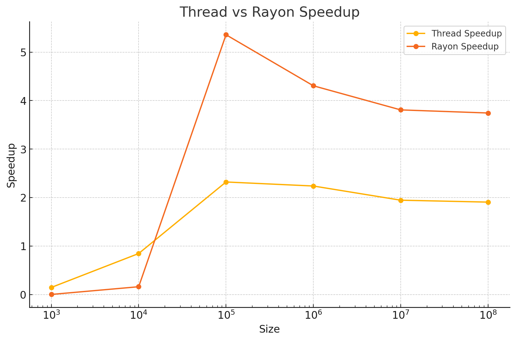
Here we can see that both methods are slower than the serial code for small amounts of work, as they are dominated by overheads. At larger problem sizes Rayon achieves close to 100% efficiency (4x speedup on 4 cores), whereas our manual approach tops out at around 50% efficiency (2x speedup on 4 threads).
Which work to parallelise?
It is common to have two possible levels over which you may wish to deploy parallelisation, consider for example this nested for loop, which estimates the proportion of prime numbers across different orders of magnitude:
fn is_prime(int: u32) -> bool {
    let upper = (int as f64).sqrt().floor() as u32;
    for div in 2..=upper {
        if int % div == 0 {
            return false;
        }
    }
    true
}
fn main() {
    let size = 20000;

    let magnitudes = vec![100000, 1000000, 10000000];
    let integers: Vec<usize> = (2..size).collect();
    // Test how many of the first `size` integers in each range are prime
    let prime_rate: Vec<f64> = magnitudes.iter().map(|mag| {
        integers.iter().map(|i| {
            if is_prime(*i as u32 + mag) {
                1.0
            } else {
                0.0
            }
        }).sum::<f64>()
    } / size as f64).collect();

    println!("{:?}", prime_rate);
}
Here there are two .iter() loops we could parallelise by replacing with .par_iter(),
the outer loop which runs three iterations over different magnitude ranges, and the inner
loop which runs 20k iterations over different integers.
Exercise Replace one of these at a time, then both, and compare the performance.
In general, parallelising the outer loop will give less of an overhead and result in better parallelisation efficiency. This is because the total work in each outer loop is necessarily larger than the work done in the inner loop.
However, if the outer loop does fewer iterations than you have cores, then efficiency will be limited. In this case, parallelising the inner loop, or possibly both loops, will be needed take advantage of the available resources.
An example of this kind of setup might be some stochastic simulations where you want to run ten repeats of everything in an inner loop, then have an outer loop over a small set of different parameter values. In this case, if you had 32 threads available you would probably want to parallelise both loops. This kind of setup also lends itself well to doing efficient parallelisation of a short inner loop with rust and rayon or C++ and OpenMP, then doing the outer parallelisation with R or python multiprocessing. Here you can even use different nodes for the outer parallelisation, assuming the computation is independent, so you might get up to 4x32 core nodes = 96 cores.
More parallelism in rust
The information in the main chapter gives most of what you'll need for easy parallel tasks in rust, which have no interdependencies or shared resources. Below we cover some more advanced use cases, although the example becomes a little more contrived.
Not covered is communication between threads. See the std::sync library
for examples, particularly the mpsc module.
Using shared memory
A real advantage of using compiled languages for parallel code is that you can easily control the memory used, and whether it is copied or not. In python and R, it is often the case that each new thread copies the memory (often the entire program's memory), which can both be slow and lead to memory use multiplying by the number of cores. On the other hand, you may need to be more careful that multiple threads aren't trying to write to the same data, or that their results may different if their execution order isn't deterministic.
Reading from shared memory without copying it is typically easy:
use std::time::Instant;
use rayon::prelude::*;
use rand::prelude::*;

fn is_prime(int: u16) -> bool {
    let upper = (int as f64).sqrt().floor() as u16;
    for div in 2..=upper {
        if int % div == 0 {
            return false;
        }
    }
    true
}
fn main() {

    let size = 20000;
    let mut rng = thread_rng();
    let mut arr = vec![0_u16; size];
    rng.fill(&mut arr[..]);

    let threads = 4;
    rayon::ThreadPoolBuilder::new().num_threads(threads).build_global().unwrap();

    let start = Instant::now();
    let integers: Vec<usize> = (0..size).collect();
    let primes: Vec<(u16, bool)> = integers.par_iter().map(|i| {
        let prime = is_prime(arr[*i] as u16);
        (arr[*i], prime)
    }).collect();

    // Timing
    let end = Instant::now();
    let parallel_time = end.duration_since(start).as_micros();
    println!("Parallel done in {}us", parallel_time);

    // Check results look ok
    println!("{:?}", &primes[0..10]);
}
In this slightly contrived example we first create random integers between 0 and \(2^{16}\)
and stored these in a Vec called arr. Each iteration then reads a position in this
list and processes it. At no point is the list copied (we didn't use .clone()).
It is also possible to write to shared memory, if you know that every thread will
write to different positions (no race conditions). One way of doing this is with .par_chunks_mut()
to make separate chunks of shared memory to write to:
#![allow(unused)]
fn main() {
use rayon::prelude::*;
use rand::prelude::*;

fn is_prime(int: u16) -> bool {
    let upper = (int as f64).sqrt().floor() as u16;
    for div in 2..=upper {
        if int % div == 0 {
            return false;
        }
    }
    true
}
// We make a list of random numbers to check whether they are prime
let size = 20000;
let mut rng = thread_rng();
let mut arr = vec![0u16; size];
rng.fill(&mut arr[..]);

// Use `iter_mut()` to split this list into non-overlapping chunks of 1000
// which we call 'slice'
let start = Instant::now();
let chunk_size = 1000;
arr.par_chunks_mut(chunk_size).for_each(|slice| {
    // Each thread iterates over its slice, if the random number is not prime
    // then we overwrite it with zero
    for int in slice.iter_mut() {
        if !is_prime(*int) {
            *int = 0;
        }
    }
});

// Check results look ok
println!("{:?}", &arr[0..10]);
}
For more complex cases where threads may write to the same location, we will need to manage these shared resources more carefully.
Managing shared memory: atomics
Let's say we now want to calculate a sum of the prime numbers up to n, with serial
code this is simple enough:
use std::time::Instant;

fn is_prime(int: u32) -> bool {
    let upper = (int as f64).sqrt().floor() as u32;
    for div in 2..=upper {
        if int % div == 0 {
            return false;
        }
    }
    true
}
fn main() {
    let size = 20000;

    let start = Instant::now();

    let integers: Vec<usize> = (2..size).collect();
    let mut sum = 0;
    integers.iter().for_each(|i| {
        if is_prime(*i as u32) {
            sum += *i;
        }
    });

    // Timing
    let end = Instant::now();
    let serial_time = end.duration_since(start).as_micros();
    println!("Serial done in {}us", serial_time);

    // Check results look ok
    println!("{sum}");
}
But if we try to replace with .par_iter() in the above code we get the following
error:
error[E0594]: cannot assign to `sum`, as it is a captured variable in a `Fn` closure
   --> src/main.rs:117:13
    |
117 |             sum += *i;
    |             ^^^^^^^^^ cannot assign

For more information about this error, try `rustc --explain E0594`.
warning: `week7` (bin "week7") generated 1 warning
rust is actually stopping us from doing this wrong. In an unsafe language we could probably use sum in this way without compiler error, but the sum would be wrong because threads would load and save to it at the same time, overwriting with the previous sum.
This would look something like this:
// thread 1                 thread 2
// read sum
// add prime1 to sum        // read sum
// write sum                // add prime2 to sum
// sum = prime1             // write sum
                            // sum = prime2
This is a type of race condition, where the order of operations affects the result, but the order is not guaranteed. So we end up with sum having missed the addition of prime1 from thread1
One way of dealing this is to make sum 'atomic', so that the load, addition, and save back to memory happen in a single unbreakable unit:
use std::time::Instant;
use std::sync::atomic::{Ordering, AtomicU32};

fn is_prime(int: u32) -> bool {
    let upper = (int as f64).sqrt().floor() as u32;
    for div in 2..=upper {
        if int % div == 0 {
            return false;
        }
    }
    true
}
fn main() {
    let size = 20000;

    let start = Instant::now();

    let integers: Vec<usize> = (2..size).collect();
    let sum = AtomicU32::new(0);
    integers.iter().for_each(|i| {
        if is_prime(*i as u32) {
            // fetch_add loads the current sum, adds the value to it, then writes
            // back to sum -- all in a single uninterruptable operation
            sum.fetch_add(*i as u32, Ordering::SeqCst);
        }
    });

    // Timing
    let end = Instant::now();
    let serial_time = end.duration_since(start).as_micros();
    println!("Atomic done in {}us", serial_time);

    // We need to use load to read from the atomic
    println!("{}", sum.load(Ordering::SeqCst));
}
If multiple threads are trying to use the atomic at the same time this will decrease efficiency as they have to wait, but typically there is a low overhead to using atomics when threads aren't in conflict.
As sums are commutative i.e. A + B = B + A so we can add the results in any order. Sums are also associative i.e. (A + B) + C = A + (B + C) so no matter which grouping of elements we sum, we can then sum these results to get a correct final sum.
This means a sum can be used as a reduction
and we could either have each thread return its own non-atomic sum, which we then add together,
or even just use the built-in .sum() operator.
Managing shared resources: mutex
What if we want to have a shared Vec which keeps track of which numbers are prime? There is
no atomic for more complex types, just the basic types (integers, floats etc). We can use
a mutal exclusion 'mutex' to protect shared data when we write to it, which works with
any type:
use std::sync::{Arc, Mutex};
use std::thread;

fn is_prime(int: u32) -> bool {
    let upper = (int as f64).sqrt().floor() as u32;
    for div in 2..=upper {
        if int % div == 0 {
            return false;
        }
    }
    true
}
fn main() {
    let size = 30;
    let primes = Arc::new(Mutex::new(Vec::new()));
    for i in 2..size {
        let list = Arc::clone(&primes);
        thread::spawn(move || {
            if is_prime(i as u32) {
                let mut list_mutex = list.lock().unwrap();
                list_mutex.push(i);
            }
        });
    }
    println!("{:?}",  primes.lock().unwrap());
}
There are a few things going on here:
- We use a
Mutexto surround theVec. - Before we can use the mutex we call
.lock()on it, this makes the thread wait until it can acquire the lock, which only a single thread can do at a time. - Calling
.lock().unwrap()allows us to write to the contained object. - The mutex is automatically unlocked when the lock goes out of scope at the end of the if statement.
- We also need to use
Arcto share (in a thread-safe way) a reference to the mutex between threads. If we don't use this we'll get a compile error as each thread will try to take control of the mutex, but only one can have mutable access in this way.
The results are correct, but might be out of order:
[2, 3, 5, 7, 13, 11, 17, 19, 23]
We are also likely to get a reduction in parallelisation efficiency as locking and unlocking the mutex takes some time, but more importantly some threads are waiting (blocking) while they wait to acquire the lock from another thread.
A typical example of a mutex might be multiple threads writing output to the terminal
writing over the top of each other, but println!()actually already guards against this with
a mutex internally.
Another use for mutex might be where each thread writes to the same file. In this
case you may want to use RwLock which
still allows reading by threads, but only one thread to have write access.
Parallelism in python
Here we will use python's multiprocessing module to use multiple cores within one
section of code.
Note that in python
threading is for async I/O and will
not make your CPU-bound code faster, whereas multiprocessing will.
Python has different executors for pools of threads and pools of processes -- see https://docs.python.org/3/library/concurrent.futures.html. In some cases one will achieve a speedup and the other won't! Typically, you should try using threads first.
On Windows and OS X python uses spawn for each
new thread, which starts a whole new python interpreter (potentially taking seconds). Unix
uses fork which is faster. Bare in mind that if you are developing software you might need to support both
methods!
We will use a python multiprocessing Pool to parallelise the outer loop of the sum_lol()
function from the optimisation chapter.
The setup is quite slow, so I will keep using numba even though it is excluded from the timing:
from numba import njit
import numpy as np
from multiprocessing import Pool
import time

@njit
def setup(N):
    xlen = N
    ylen = N

    rand_mat = np.random.rand(xlen, ylen)

    lol = list()
    for x in range(xlen):
        sublist = list()
        for y in range(ylen):
            sublist.append(rand_mat[x, y])
        lol.append(sublist)
    return lol

# Serial version
def sum_lol(lol):
    sum = 0
    for x in range(len(lol)):
        for y in range(len(lol[x])):
            sum += lol[x][y]
    return sum

# Parallel map which sums one sublist
def sum_list(sublist):
    partial_sum = 0
    for entry in sublist:
        partial_sum += entry
    return partial_sum

def run_test(N, threads):
    lol = setup(N)
    start_t = time.time_ns()

    if threads > 1:
        # map
        with Pool(processes=threads) as pool:
            partial_sums = pool.map(sum_list, lol)
        # reduce
        final_sum = sum_list(partial_sums)
    else:
        final_sum = sum_lol(lol)

    end_t = time.time_ns()
    time_ms = (end_t - start_t) / 1000000

    print(f"Time to sum {N**2} entries with {threads} threads: {time_ms}ms")

def main():
    for threads in range(1, 5):
        for N_exp in range(5):
            run_test(10**(N_exp), threads)

if __name__ == "__main__":
    main()
Exercise What is the speedup and efficiency? Plot this as the size of the list grows, and varying the size of the pool.
Parallel sum solution
On OS X, this gives me the following:
Time to sum 1 entries with 1 threads: 0.004ms
Time to sum 100 entries with 1 threads: 0.009ms
Time to sum 10000 entries with 1 threads: 0.63ms
Time to sum 1000000 entries with 1 threads: 66.252ms
Time to sum 100000000 entries with 1 threads: 6856.647ms
Time to sum 1 entries with 2 threads: 369.239ms
Time to sum 100 entries with 2 threads: 350.236ms
Time to sum 10000 entries with 2 threads: 344.328ms
Time to sum 1000000 entries with 2 threads: 378.785ms
Time to sum 100000000 entries with 2 threads: 4554.182ms
Time to sum 1 entries with 3 threads: 372.856ms
Time to sum 100 entries with 3 threads: 360.495ms
Time to sum 10000 entries with 3 threads: 361.229ms
Time to sum 1000000 entries with 3 threads: 384.375ms
Time to sum 100000000 entries with 3 threads: 3399.802ms
Time to sum 1 entries with 4 threads: 394.478ms
Time to sum 100 entries with 4 threads: 375.59ms
Time to sum 10000 entries with 4 threads: 388.037ms
Time to sum 1000000 entries with 4 threads: 425.455ms
Time to sum 100000000 entries with 4 threads: 2956.621ms
For smaller lists, the time is always around 300-400ms on any multithreaded
implementation, which is just the overhead of creating the Pool. For the larger
list more threads is giving more speed, at around 75% efficiency for two threads,
reducing to around 60% efficiency with four threads.
Here we are running a thread for each go around the outer loop, i.e. for x in range(len(lol)).
We could also run threads to parallelise the inner loop too. What would be the advantages
and disadvantages of this approach?
Returning results and shared memory
The above example is simple in that the function being parallelised takes a single
iteraable and returns a single value (a scalar), so the return from Pool.map is a list of these scalars.
If you want to run a function which has other arguments, you can use partial to bind the other arguments before passing it as a closure
to the map call.
If you want each thread to write results into (non-overlapping) parts of shared memory
this is possible with SharedMemory
introduced in python 3.8. This is also useful if you have very large arrays as input
which would otherwise be copied across every thread increasing memory use.
We won't go into this much further, but here is an example of putting all of this together which assigns samples to a HDBSCAN model in parallel:
# Imports
from functools import partial
from tqdm.contrib.concurrent import thread_map, process_map
try:
    from multiprocessing import shared_memory
    from multiprocessing.managers import SharedMemoryManager
    NumpyShared = collections.namedtuple('NumpyShared', ('name', 'shape', 'dtype'))
except ImportError as e:
    sys.stderr.write("This code requires python v3.8 or higher\n")
    sys.exit(0)

def assign_samples(chunk, X, y, model, n_samples, chunk_size):
    # Load in shared memory
    if isinstance(X, NumpyShared):
        X_shm = shared_memory.SharedMemory(name = X.name)
        X = np.ndarray(X.shape, dtype = X.dtype, buffer = X_shm.buf)
    if isinstance(y, NumpyShared):
        y_shm = shared_memory.SharedMemory(name = y.name)
        y = np.ndarray(y.shape, dtype = y.dtype, buffer = y_shm.buf)

    # Set range thread is operating on
    start = chunk * chunk_size
    end = min((chunk + 1) * chunk_size, n_samples)

    # Run the prediction for this range
    y[start:end] = hdbscan.approximate_predict(model.hdb, X[start:end, :])[0]

# Set output to zeros
y = np.zeros(n_samples, dtype=int)
block_size = 100000
with SharedMemoryManager() as smm:
    # Make a shared memory array for input X and copy data into it
    shm_X = smm.SharedMemory(size = X.nbytes)
    X_shared_array = np.ndarray(X.shape, dtype = X.dtype, buffer = shm_X.buf)
    X_shared_array[:] = X[:]
    X_shared = NumpyShared(name = shm_X.name, shape = X.shape, dtype = X.dtype)

    # Make a share memory array for output y and copy data into it
    shm_y = smm.SharedMemory(size = y.nbytes)
    y_shared_array = np.ndarray(y.shape, dtype = y.dtype, buffer = shm_y.buf)
    y_shared_array[:] = y[:]
    y_shared = NumpyShared(name = shm_y.name, shape = y.shape, dtype = y.dtype)

    # Run the function `assign_sample` multithreaded
    thread_map(partial(assign_samples,
                                X = X_shared,
                                y = y_shared,
                                model = dbscan_model,
                                n_samples = n_samples,
                                chunk_size = block_size),
                        range((n_samples - 1) // block_size + 1),
                        max_workers=threads)

    # Copy results back into y
    y[:] = y_shared_array[:]

return y
Notes:
thread_mapfromtqdmis used, to provide a progress bar.partialis used to bind the arguments ofassign_samples, as the map only iterates over the first argument.- A
SharedMemoryManageris used to share numpy arrays between threads without copying them. - The main code needs to set these arrays up using a buffer.
- The called function needs to unpack them.
- Non-overlapping rows of the array each thread operates on are manually calculated.
Parallelism in R
Contents:
There are a few different libraries in R which can help parallelise code. Let's consider a new example of calculating the volume of an N-dimensional hypersphere with Monte Carlo:
sphere_volume <- function(steps, dimension) {
  in_hypersphere <- 0
  for (n in 1:steps) {
    coordinates <- runif(dimension, min = -1, max = 1)
    if (sum(coordinates ** 2) < 1) {
      in_hypersphere <- in_hypersphere + 1
    }
  }
  2 ** dimension * in_hypersphere / steps
}
This uses the idea that we can calculate the volume of a hypercube in N-dimensions with sides of length two by \( 2^N \). Inside that hypercube, we can fit a hypersphere with radius \(r = 1\). If we randomly generate points inside the hypercube, and count the proportion which are inside the hypersphere, we will get the ratio of the volume of the hypersphere to the hypercube, so can calculate the hypersphere volume with: \[ V_{\mathrm{sphere}} = V_{\mathrm{cube}} * \frac{\mathrm{draw}_\mathrm{inside}}{\mathrm{draw} _ \mathrm{total}} \] Making draws between -1 and 1 for each dimension will be within the cube. We can then use Pythagoras to determine whether draws are inside the sphere: \[ r^2 < x^2 + y^2 + z^2 + ...\]
See the wikipedia page on Monte Carlo integration for more info and drawings.
Exercise: We know the formulae for a 2D-sphere (circle) and 3D sphere. Run the above function and verify the result.
Using parallel::mclapply
The 2D example is an estimate of \( \pi \), but a slowly converging one. The error goes down only by \( \frac{1}{\sqrt N} \), so we need many samples to get a good estimate. Using \(10^7 \) samples takes around 10s, but only gets the first four digits correct.
These samples are totally independent, so they should be easy to parallelise, right? Let's first use a parallel version of lapply:
sphere_volume <- function(steps, dimension) {
  in_hypersphere <- 0
  for (n in 1:steps) {
    coordinates <- runif(dimension, min = -1, max = 1)
    if (sum(coordinates ** 2) < 1) {
      in_hypersphere <- in_hypersphere + 1
    }
  }
  2 ** dimension * in_hypersphere / steps
}

steps <- 10000000
dimension <- 2
system.time(sphere_volume(steps, dimension)) # 7.258s

cores <- 4
system.time(mean(unlist(parallel::mclapply(rep(10000000/cores, cores), sphere_volume, 2, mc.cores = cores))))
# 2.211s
# Speedup =~3.3x
Similar to writing rust code using iterables, it's often better to write R code by applying functions to lists or arrays. This is true even in serial R code, as it can vectorise operations. Here we divide the work (the draws) equally among the cores, making a list with the number of steps that each thread will compute. We can then calculate the average of the estimate from each core. Though, it may be more precise to return the number of draws inside the circle as an integer and sum these, then do the division once at the end.
What happens if you add set.seed(1) in the function?
All of the estimates are the same, because the random draws are the same. We are using a pseudorandom number generator (RNG), which given the same starting state will generate the same sequence of numbers.
You can achieve the same by adding mc.set.seed = FALSE to mclapply, which shares
the same RNG state when the threads are forked. The default of TRUE will set a seed based on the time and process ID,
which will likely give a different set of random numbers on each thread. If you want
your results to be reproducible, you'd want to manually set a consistent seed e.g. using the thread index
at the top of the sphere_volume function.
But note, for very long streams (or if you are unlucky) these numbers may start to overlap! There are true parallel random number generators which solve this (rust has these). See Figure 3 of this paper for an illustration of this.
Using foreach and doParallel
We can also parallelise for loops more directly using the dopar operator:
library(doParallel)
library(foreach)

cores <- 4
registerDoParallel(cores)

sphere_volume <- function(steps, dimension) {
  in_hypersphere <- foreach (n=1:steps, .combine = '+') %dopar% {
    coordinates <- runif(dimension, min = -1, max = 1)
    if (sum(coordinates ** 2) <= 1) {
      1
    }
  }
  2 ** dimension * in_hypersphere / steps
}
steps <- 10000000
dimension <- 2
system.time(sphere_volume(steps, dimension)) # dnf after 30s
Here using a sum reduction to count the number of points in the circle. This doesn't parallelise particularly well at all (small amount of work on lots of threads), and didn't even finish for me.
Dividing the work up manually with a parallelised outer loop works a lot better:
library(doParallel)
library(foreach)

cores <- 4
registerDoParallel(cores)

sphere_volume <- function(steps, dimension, cores) {
  # Outer loop parallelised over cores, sum results
  total_count <- foreach (n=1:cores, .combine = '+') %dopar% {
    set.seed(n)
    in_hypersphere <- 0
    # Inner loop run on each thread
    for (i in 1:(steps/cores)) {
      coordinates <- runif(dimension, min = -1, max = 1)
      if (sum(coordinates ** 2) <= 1) {
        in_hypersphere <- in_hypersphere + 1
      }
    }
    in_hypersphere
  }
  2 ** dimension * total_count / steps
}

steps <- 10000000
dimension <- 2
system.time(sphere_volume(steps, dimension, cores)) # 2.05s
This gave a ~3.7x speedup, a bit better than mclapply.
Parallel R using furrr
Finally, if you are a fan of tidyverse type R and functional programming with purrr,
there is a parallel version called furrr.
This gives you a parallel version of .map(), which is similar to the rust iterators,
and looks quite similar to lapply.
Here it is with the integration example:
library(furrr)
library(purrr)

# Various different ways to parallelise are supported
cores <- 4
plan(multisession, workers = cores)

sphere_volume <- function(steps, dimension) {
  in_hypersphere <- 0
  for (n in 1:steps) {
    coordinates <- runif(dimension, min = -1, max = 1)
    if (sum(coordinates ** 2) < 1) {
      in_hypersphere <- in_hypersphere + 1
    }
  }
  2 ** dimension * in_hypersphere / steps
}

steps <- 10000000
dimension <- 2
# future_map_dbl returns a vector of doubles (decimal numbers), which is applied
# the same way as the mclapply example above.
# future_<> is the purrr (parallel) version of functions from furrr
# We also set the seed in a similar way
system.time(mean(future_map_dbl(rep(steps/cores, cores),
                                sphere_volume, dimension,
                                .options=furrr_options(seed=TRUE))))
# 2.743s
This gives me a speedup of ~2.6x with multicore, or ~3.1x with multisession and cluster.