Optimising python code

Some guiding principles:

Only optimise code if you need to. By optimising it, will it be able to run on something you couldn't analyse otherwise? Will it save you more computation than the time it takes to optimise? Will lots of other people use the code, and therefore collectively save time?
In my experience, going after >10x speedups is usually worth it as it hits the first two objectives. Going after ~2x speedups can often be worth it for commonly used programs, or that you intend to distribute as software. A 10% speedup is rarely worth it for research code -- this would be useful in library code used by thousands of people.
Get the code to work before optimising it. It's helpful to have a test to ensure any changes you make haven't broken anything.
Do your optimisation empirically, i.e. use a profiler. We're pretty bad at working out by intuition where the slow parts of the code are.

For now, we'll focus on a python example, but the ideas are similar in R.

Counting codons
- Aside: debugging
Profiling
Optimisation strategies
Memory optimisation
Writing extensions in compiled code
Other optimisations
Notes (for next year)

Counting codons

The first example we will work through is counting codons from a multiple sequence alignment.

A multiple sequence alignment stored in FASTA format might look something like:

>ERR016988;0_0_13
atgaaaaacactatgtctcctaaaaaaatacccatttggcttaccggcctcatcctactg
attgccctaccgcttaccctgccttttttatatgtcgctatgcgttcgtggcaggtcggc
atcaaccgcgccgtcgaactgttgttccgcccgcgtatgtgggatttgctctccaacacc
ttgacgatgatggcgggcgttaccctgatttccattgttttgggcattgcctgctccctt
ttgttccaacgttaccgcttcttcggcaaaaccttttttcagacggcaatcaccctgcct
ttgtgcatccccgcatttgtcagctgtttcacctggatcagcctgaccttccgtgtcgaa
ggcttttgggggacagtgatgattatgagcctgtcctcgttcccgctcgcctacctgccc
gtcgaggcggcactcaaacgcatcagcctgtcttacgaagaagtcagcctgtccttgggc
aaaagccgcctgcaaacctttttttccgccatcctcccccagctcaaacccgccatcggc
agcagcgtgttactgattgccctgcatatgctggtcgaatttggcgcggtatccattttg
aactaccccacttttaccaccgccattttccaagaatacgaaatgtcctacaacaacaat
accgccgccctgctttccgctgttttaatggcggtgtgcggcatcgtcgtatttggagaa
agcatatttcgcggcaaagccaagatttaccacagcggcaaaggcgttgcccgtccttat
cccgtcaaaaccctcaaactgcccggtcagattggcgcgattgtttttttaagcagcttg
ttgactttgggcattattatcccctttggcgtattgatacattggatgatggtcggcact
tccggcacattcgcgctcgtatccgtatttgatgcctttatccgttccttaagcgtatcg
gctttaggtgcgattttgactatattatgtgccttgccccttgtttgggcatcggttcgc
tatcgcaattttttaaccgtttggatagacaggctgccgtttttactgcacgccgtcccc
ggtttggttatcgccctatccttggtttatttcagcatcaactacacccctgccgtttac
caaacctttatcgtcgtcatccttgcctatttcatgctttacctgccgatggcgcaaacc
accctgaggacttccttggaacaactccccaaagggatggaacaggtcggcgcaacattg
gggcgcggacacttctttattttcaggacgttggtactgccgtccatcctgcccggcatt
accgccgcattcgcactcgtcttcctcaaactgatgaaagagctgaccgccaccctgctg
ctgaccaccgacgatgtccacacactctccaccgccgtttgggaatacacatcggacgca
caatacgccgccgccaccccttacgcgctgatgctggtattattttccggcatccccgta
ttcctgctgaagaaatacgccttcaaataa------------------------
>ERR016989;1_112_17
atgaaaaacactatgtctcctaaaaaaatacccatttggcttaccggcctcatcctactg
attgccctaccgcttaccctgccttttttatatgtcgctatgcgttcgtggcaggtcggc
atcaaccgcgccgtcgaactgttgttccgcccgcgtatgtgggatttgctctccaacacc
ttgacgatgatggcgggcgttaccctgatttccattgttttgggcattgcctgcgccctt
ttgttccaacgttaccgcttcttcggcaaaaccttttttcagacggcaatcaccctgcct
ttgtgcatccccgcatttgtcagctgtttcacctggatcagcctgaccttccgtgtcgaa
ggcttttgggggacagtgatgattatgagcctgtcctcgttcccgctcgcctacctgccc
gtcgaggcggcactcaaacgcatcagcctgtcttacgaagaagtcagcctgtccttgggc
aaaagccgcctgcaaacctttttttccgccatcctcccccagctcaaacccgccatcggc
agcagcgtgttactgattgccctgcatatgctggtcgaatttggcgcggtatccattttg
aactaccccacttttaccaccgccattttccaagaatacgaaatgtcctacaacaacaat
accgccgccctgctttccgctgttttaatggcggtgtgcggcatcgtcgtatttggagaa
agcatatttcgcggcaaagccaagatttaccacagcggcaaaggcgttgcccgtccttat
cccgtcaaaaccctcaacctccccggtcagattggcgcgattgtttttttaagcagcttg
ttgactttgggcattattatcccctttggcgtattgatacattggatgatggtcggcact
tccggcacattcgcgctcgtatccgtatttgatgcctttatccgttccttaagcgtatcg
gctttaggtgcggttttgactatattatgtgccttgccccttgtttgggcatcggtccgc
tatcgcaattttttaaccgtttggatagacaggctgccgtttttactgcacgccgtcccc
ggtttggttatcgccctatccttggtttatttcagcatcaactacacccctgccgtttac
caaacctttatcgtcgtcatccttgcctatttcatgctttacctgccgatggcgcaaacc
accctaaggacttccttggaacaactcccaaaagggatggaacaggtcggcgcaacattg
gggcgcggacacttctttattttcaggacgttggtactgccgtccatcctgcccggcatt
accgccgcattcgcactcgtcttcctcaaactgatgaaagagctgaccgccaccctgctg
ctgaccaccgacgatgtccacacactctccaccgccgtttgggaatacacatcggacgca
caatacgccgccgccaccccttacgcgctgatgctggtattattttccggcatccccgta
ttcctgctgaagaaatacgctttcaaataa------------------------

This format has sample headers which start > followed by the sample name, followed by the sequence, wrapped at 80 characters to make it more human readable. Gaps are given by - characters. We wish to count, at each aligned position, the number of observed codons for each of the 61 possible triplet positions plus the three stop codons TAG, TAA and TGA.

We'll use an example with aligned porB sequences from the bacterial pathogen Neisseria meningitidis, which you can download here.

Exercise Let's start off by writing some code in to read this file in and doing a simple check that the length is as expected (all the same, and a multiple of three). Let's also add some timing in, to see if we are improving when we add optimisations.

Have a go at this yourself, and then compare with the example below.

Example: read file

import time
import gzip

# Generator which keeps state after yield is called
# Based on a nice example: https://stackoverflow.com/a/7655072
def read_fasta_sample(fp):
    name, seq = None, []
    for line in fp:
        line = line.rstrip()
        if line.startswith(">"):
            if name: yield (name, ''.join(seq).upper())
            name, seq = line[1:], []
        else:
            seq.append(line)
    if name: yield (name, ''.join(seq).upper())

def read_file(file_name):
    n_samples = 0
    # Open either gzipped or plain file by looking for magic number
    # https://stackoverflow.com/a/47080739
    with open(file_name, 'rb') as test_f:
        zipped = test_f.read(2) == b'\x1f\x8b'
    if zipped:
        fh = gzip.open(file_name, 'rt')
    else:
        fh = open(file_name, 'rt')
    with fh as fasta:
        seqs = list()
        names = list()
        for h, s in read_fasta_sample(fasta):
            if len(s) % 3 != 0:
                raise RuntimeError(f"Sequence {h} is not a multiple of three")
            elif len(seqs) > 0 and len(s) != len(seqs[0]):
                raise RuntimeError(f"Sequence {h} is length {len(s)}, expecting {len(seqs[0])}")
            else:
                seqs.append(s)
                names.append(h)

    return seqs, names

def main():
    start_t = time.time_ns()
    seqs, names = read_file("BIGSdb_024538_1190028856_31182.dna.aln.gz")
    end_t = time.time_ns()
    time_ms = (end_t - start_t) / 1000000
    print(f"Time to read {len(seqs)} samples: {time_ms}ms")

if __name__ == "__main__":
    main()

Don't worry about perfecting your code at this point! Let's aim for something that runs easily and works, which we can then improve if we end up using it.

In the example above I have added a timer so we can try and keep track of how long each section takes to run. A better way to do this would be to average over multiple runs, for example using the timeit module, but some measurement is better than no measurement.

I've made sure all the bases are uppercase so we don't have to deal with both a and A in our counter, but I haven't checked for incorrect bases.

When I run this code, I see the following:

python example1.py
Time to read 4889 samples: 59.502ms

If I decompress the file first:

python example1.py
Time to read 4889 samples: 33.419ms

If you have a hard disk drive rather than a solid state drive, it is often faster to read compressed data and decompress it on the fly, as the speed of data transfer is the rate limiting step.

Exercise Now, using the sequences, write some code to actually count the codons. The output should be a frequency vector at every site for every codon which does not contain a -. Do this however you like.

Example: count codons

def count_codons(seqs):
    bases = ['A', 'C', 'G', 'T']
    codon_len = int(len(seqs[0]) // 3)
    counts = [dict()] * codon_len
    for seq in seqs:
        for codon_idx in range(codon_len):
            nuc_idx = codon_idx * 3
            codon = seq[nuc_idx:(nuc_idx + 3)]
            if all([base in bases for base in codon]):
                if codon in counts[codon_idx]:
                    counts[codon_idx][codon] += 1
                else:
                    counts[codon_idx][codon] = 1

    count_vec = list()
    for pos in counts:
        pos_vec = list()
        for base1 in bases:
            for base2 in bases:
                for base3 in bases:
                    codon = ''.join(base1 + base2 + base3)
                    if codon in pos:
                        pos_vec.append(pos[codon])
                    else:
                        pos_vec.append(0)

    return count_vec

Aside: debugging

My first attempt (above) was wrong and was returning an empty list. One way to look into this is by using a debugger.

Modern IDEs such as vscode and pycharm also let you run the debugger interactively, which is typically nicer than via the command line. However old school debugging is handy when you have to run your code on HPC systems, or with more complex projects such as when you have C++ and python code interacting.

python has pdb built-in, you can run it as follows:

python -m pdb example1.py

(gdb and lldb are equivalent debuggers for compiled code.)

Run help to see the commands. Most useful are setting breakpoints with b; continuing execution with c, r, s and n; printing variables with p.

By stopping my code on the line with codon = ''.join(base1 + base2 + base3) by typing b 62 to add a breakpoint, then r to run the code, I can have a look at some counts:

p pos
{'ATG': 15401, 'TGA': 47348, 'GAA': 39489, 'AAA': 85118, 'AAT': 30105, 'ATC': 36135, 'TCC': 24440, 'CCC': 22958, 'CCT': 36610, 'CTG': 41756, 'GAT': 10002, 'ATT': 20458, 'TTG': 49731, 'TGC': 21500, 'GCC': 40734, 'GAC': 20218, 'ACT': 19778, 'CTT': 28321, 'TTT': 20797, 'TGG': 29906, 'GGC': 67370, 'GCA': 45599, 'CAG': 23779, 'AGC': 34794, 'TTC': 29469, 'TGT': 9964, 'GTT': 39620, 'CAA': 42858, 'GCT': 30373, 'ACG': 15084, 'CGT': 23916, 'TTA': 9198, 'TAC': 21812, 'ACC': 30370, 'GTA': 33903, 'CGG': 62505, 'CAC': 11408, 'CCA': 20119, 'CAT': 22822, 'TCA': 20719, 'AAG': 42061, 'CCG': 35604, 'GCG': 24592, 'TAG': 10002, 'AGA': 17961, 'AAC': 28534, 'CGC': 21035, 'CTC': 19077, 'TCT': 13737, 'GAG': 4230, 'ACA': 15865, 'GGA': 5578, 'GGT': 42665, 'GTC': 11842, 'AGG': 21378, 'GTG': 1830, 'TCG': 37628, 'GGG': 13214, 'TAA': 18253, 'CTA': 9810, 'TAT': 6398, 'ATA': 2220, 'CGA': 5452, 'AGT': 5939}

For starters, these seem far too high, as we wouldn't expect counts over the number of samples (4889).

Stopping at codon = seq[codon_idx:(codon_idx + 3)] I see:

(Pdb) p codon
'ATG'

This looks ok. I'll step through some of the next lines with n:

if codon in counts[codon_idx]:
(Pdb) p counts
[{}, {}, {}, {}, {}, {}, {}, {}, {}, {}, {}, {}, {}, {}, {}, {}, {}, {}, {}, {}, {}, {}, {}, {}, {}, {}, {}, {}, {}, {}, {}, {}, {}, {}, {}, {}, {}, {}, {}, {}, {}, {}, {}, {}
, {}, {}, {}, {}, {}, {}, {}, {}, {}, {}, {}, {}, {}, {}, {}, {}, {}, {}, {}, {}, {}, {}, {}, {}, {}, {}, {}, {}, {}, {}, {}, {}, {}, {}, {}, {}, {}, {}, {}, {}, {}, {}, {}, {
}, {}, {}, {}, {}, {}, {}, {}, {}, {}, {}, {}, {}, {}, {}, {}, {}, {}, {}, {}, {}, {}, {}, {}, {}, {}, {}, {}, {}, {}, {}, {}, {}, {}, {}, {}, {}, {}, {}, {}, {}, {}, {}, {},
{}, {}, {}, {}, {}, {}, {}, {}, {}, {}, {}, {}, {}, {}, {}, {}, {}, {}, {}, {}, {}, {}, {}, {}, {}, {}, {}, {}, {}, {}, {}, {}, {}, {}, {}, {}, {}, {}, {}, {}, {}, {}, {}, {},
 {}, {}, {}, {}, {}, {}, {}, {}, {}, {}, {}, {}, {}, {}, {}, {}, {}, {}, {}, {}, {}, {}, {}, {}, {}, {}, {}, {}, {}, {}, {}, {}, {}, {}, {}, {}, {}, {}, {}, {}, {}, {}, {}, {}
, {}, {}, {}, {}, {}, {}, {}, {}, {}, {}, {}, {}, {}, {}, {}, {}, {}, {}, {}, {}, {}, {}, {}, {}, {}, {}, {}, {}, {}, {}, {}, {}, {}, {}, {}, {}, {}, {}, {}, {}, {}, {}, {}, {
}, {}, {}, {}, {}, {}, {}, {}, {}, {}, {}, {}, {}, {}, {}, {}, {}, {}, {}, {}, {}, {}, {}, {}, {}, {}, {}, {}, {}, {}, {}, {}, {}, {}, {}, {}, {}, {}, {}, {}, {}, {}, {}, {},
{}, {}, {}, {}, {}, {}, {}, {}, {}, {}, {}, {}, {}, {}, {}, {}, {}, {}, {}, {}, {}, {}, {}, {}, {}, {}, {}, {}, {}, {}, {}, {}, {}, {}, {}, {}, {}, {}, {}, {}, {}, {}, {}, {},
 {}, {}, {}, {}, {}, {}, {}, {}, {}, {}, {}, {}, {}, {}, {}, {}, {}, {}, {}, {}, {}, {}, {}, {}, {}, {}, {}, {}, {}, {}, {}, {}, {}, {}, {}, {}, {}, {}, {}, {}, {}, {}, {}, {}
, {}, {}, {}, {}, {}, {}, {}, {}, {}]

Initialisation looks ok

> example1.py(51)count_codons()
-> counts[codon_idx][codon] = 1
(Pdb) n
> example1.py(45)count_codons()
-> for codon_idx in range(codon_len):
(Pdb) p counts
[{'ATG': 1}, {'ATG': 1}, {'ATG': 1}, {'ATG': 1}, {'ATG': 1}, {'ATG': 1}, {'ATG': 1}, {'ATG': 1}, {'ATG': 1}, {'ATG': 1}, {'ATG': 1}, {'ATG': 1}, {'ATG': 1}, {'ATG': 1}, {'ATG'
: 1}, {'ATG': 1}, {'ATG': 1}, {'ATG': 1}, {'ATG': 1}, {'ATG': 1}, {'ATG': 1}, {'ATG': 1}, {'ATG': 1}, {'ATG': 1}, {'ATG': 1}, {'ATG': 1}, {'ATG': 1}, {'ATG': 1}, {'ATG': 1}, {
'ATG': 1}, {'ATG': 1}, {'ATG': 1}, {'ATG': 1}, {'ATG': 1}, {'ATG': 1}, {'ATG': 1}, {'ATG': 1}, {'ATG': 1}, {'ATG': 1}, {'ATG': 1}, {'ATG': 1}, {'ATG': 1}, {'ATG': 1}, {'ATG':
1}, {'ATG': 1}, {'ATG': 1}, {'ATG': 1}, {'ATG': 1}, {'ATG': 1}, {'ATG': 1}, {'ATG': 1}, {'ATG': 1}, {'ATG': 1}, {'ATG': 1}, {'ATG': 1}, {'ATG': 1}, {'ATG': 1}, {'ATG': 1}, {'A
TG': 1}, {'ATG': 1}, {'ATG': 1}, {'ATG': 1}, {'ATG': 1}, {'ATG': 1}, {'ATG': 1}, {'ATG': 1}, {'ATG': 1}, {'ATG': 1}, {'ATG': 1}, {'ATG': 1}, {'ATG': 1}, {'ATG': 1}, {'ATG': 1}
, {'ATG': 1}, {'ATG': 1}, {'ATG': 1}, {'ATG': 1}, {'ATG': 1}, {'ATG': 1}, {'ATG': 1}, {'ATG': 1}, {'ATG': 1}, {'ATG': 1}, {'ATG': 1}, {'ATG': 1}, {'ATG': 1}, {'ATG': 1}, {'ATG
': 1}, {'ATG': 1}, {'ATG': 1}, {'ATG': 1}, {'ATG': 1}, {'ATG': 1}, {'ATG': 1}, {'ATG': 1}, {'ATG': 1}, {'ATG': 1}, {'ATG': 1}, {'ATG': 1}, {'ATG': 1}, {'ATG': 1}, {'ATG': 1},
{'ATG': 1}, {'ATG': 1}, {'ATG': 1}, {'ATG': 1}, {'ATG': 1}, {'ATG': 1}, {'ATG': 1}, {'ATG': 1}, {'ATG': 1}, {'ATG': 1}, {'ATG': 1}, {'ATG': 1}, {'ATG': 1}, {'ATG': 1}, {'ATG':
 1}, {'ATG': 1}, {'ATG': 1}, {'ATG': 1}, {'ATG': 1}, {'ATG': 1}, {'ATG': 1}, {'ATG': 1}, {'ATG': 1}, {'ATG': 1}, {'ATG': 1}, {'ATG': 1}, {'ATG': 1}, {'ATG': 1}, {'ATG': 1}, {'
ATG': 1}, {'ATG': 1}, {'ATG': 1}, {'ATG': 1}, {'ATG': 1}, {'ATG': 1}, {'ATG': 1}, {'ATG': 1}, {'ATG': 1}, {'ATG': 1}, {'ATG': 1}, {'ATG': 1}, {'ATG': 1}, {'ATG': 1}, {'ATG': 1
}, {'ATG': 1}, {'ATG': 1}, {'ATG': 1}, {'ATG': 1}, {'ATG': 1}, {'ATG': 1}, {'ATG': 1}, {'ATG': 1}, {'ATG': 1}, {'ATG': 1}, {'ATG': 1}, {'ATG': 1}, {'ATG': 1}, {'ATG': 1}, {'AT
G': 1}, {'ATG': 1}, {'ATG': 1}, {'ATG': 1}, {'ATG': 1}, {'ATG': 1}, {'ATG': 1}, {'ATG': 1}, {'ATG': 1}, {'ATG': 1}, {'ATG': 1}, {'ATG': 1}, {'ATG': 1}, {'ATG': 1}, {'ATG': 1},
 {'ATG': 1}, {'ATG': 1}, {'ATG': 1}, {'ATG': 1}, {'ATG': 1}, {'ATG': 1}, {'ATG': 1}, {'ATG': 1}, {'ATG': 1}, {'ATG': 1}, {'ATG': 1}, {'ATG': 1}, {'ATG': 1}, {'ATG': 1}, {'ATG'
: 1}, {'ATG': 1}, {'ATG': 1}, {'ATG': 1}, {'ATG': 1}, {'ATG': 1}, {'ATG': 1}, {'ATG': 1}, {'ATG': 1}, {'ATG': 1}, {'ATG': 1}, {'ATG': 1}, {'ATG': 1}, {'ATG': 1}, {'ATG': 1}, {
'ATG': 1}, {'ATG': 1}, {'ATG': 1}, {'ATG': 1}, {'ATG': 1}, {'ATG': 1}, {'ATG': 1}, {'ATG': 1}, {'ATG': 1}, {'ATG': 1}, {'ATG': 1}, {'ATG': 1}, {'ATG': 1}, {'ATG': 1}, {'ATG':
1}, {'ATG': 1}, {'ATG': 1}, {'ATG': 1}, {'ATG': 1}, {'ATG': 1}, {'ATG': 1}, {'ATG': 1}, {'ATG': 1}, {'ATG': 1}, {'ATG': 1}, {'ATG': 1}, {'ATG': 1}, {'ATG': 1}, {'ATG': 1}, {'A
TG': 1}, {'ATG': 1}, {'ATG': 1}, {'ATG': 1}, {'ATG': 1}, {'ATG': 1}, {'ATG': 1}, {'ATG': 1}, {'ATG': 1}, {'ATG': 1}, {'ATG': 1}, {'ATG': 1}, {'ATG': 1}, {'ATG': 1}, {'ATG': 1}
, {'ATG': 1}, {'ATG': 1}, {'ATG': 1}, {'ATG': 1}, {'ATG': 1}, {'ATG': 1}, {'ATG': 1}, {'ATG': 1}, {'ATG': 1}, {'ATG': 1}, {'ATG': 1}, {'ATG': 1}, {'ATG': 1}, {'ATG': 1}, {'ATG
': 1}, {'ATG': 1}, {'ATG': 1}, {'ATG': 1}, {'ATG': 1}, {'ATG': 1}, {'ATG': 1}, {'ATG': 1}, {'ATG': 1}, {'ATG': 1}, {'ATG': 1}, {'ATG': 1}, {'ATG': 1}, {'ATG': 1}, {'ATG': 1},
{'ATG': 1}, {'ATG': 1}, {'ATG': 1}, {'ATG': 1}, {'ATG': 1}, {'ATG': 1}, {'ATG': 1}, {'ATG': 1}, {'ATG': 1}, {'ATG': 1}, {'ATG': 1}, {'ATG': 1}, {'ATG': 1}, {'ATG': 1}, {'ATG':
 1}, {'ATG': 1}, {'ATG': 1}, {'ATG': 1}, {'ATG': 1}, {'ATG': 1}, {'ATG': 1}, {'ATG': 1}, {'ATG': 1}, {'ATG': 1}, {'ATG': 1}, {'ATG': 1}, {'ATG': 1}, {'ATG': 1}, {'ATG': 1}, {'
ATG': 1}, {'ATG': 1}, {'ATG': 1}, {'ATG': 1}, {'ATG': 1}, {'ATG': 1}, {'ATG': 1}, {'ATG': 1}, {'ATG': 1}, {'ATG': 1}, {'ATG': 1}, {'ATG': 1}, {'ATG': 1}, {'ATG': 1}, {'ATG': 1
}, {'ATG': 1}, {'ATG': 1}, {'ATG': 1}, {'ATG': 1}, {'ATG': 1}, {'ATG': 1}, {'ATG': 1}, {'ATG': 1}, {'ATG': 1}, {'ATG': 1}, {'ATG': 1}, {'ATG': 1}, {'ATG': 1}, {'ATG': 1}, {'AT
G': 1}, {'ATG': 1}, {'ATG': 1}, {'ATG': 1}, {'ATG': 1}, {'ATG': 1}, {'ATG': 1}, {'ATG': 1}, {'ATG': 1}, {'ATG': 1}, {'ATG': 1}, {'ATG': 1}, {'ATG': 1}, {'ATG': 1}, {'ATG': 1},
 {'ATG': 1}, {'ATG': 1}, {'ATG': 1}, {'ATG': 1}, {'ATG': 1}, {'ATG': 1}, {'ATG': 1}, {'ATG': 1}, {'ATG': 1}, {'ATG': 1}, {'ATG': 1}, {'ATG': 1}, {'ATG': 1}, {'ATG': 1}, {'ATG'
: 1}, {'ATG': 1}, {'ATG': 1}, {'ATG': 1}, {'ATG': 1}, {'ATG': 1}, {'ATG': 1}, {'ATG': 1}, {'ATG': 1}, {'ATG': 1}, {'ATG': 1}, {'ATG': 1}, {'ATG': 1}, {'ATG': 1}, {'ATG': 1}, {
'ATG': 1}, {'ATG': 1}, {'ATG': 1}, {'ATG': 1}, {'ATG': 1}, {'ATG': 1}, {'ATG': 1}, {'ATG': 1}, {'ATG': 1}, {'ATG': 1}, {'ATG': 1}, {'ATG': 1}, {'ATG': 1}, {'ATG': 1}, {'ATG':
1}, {'ATG': 1}, {'ATG': 1}, {'ATG': 1}, {'ATG': 1}, {'ATG': 1}, {'ATG': 1}, {'ATG': 1}, {'ATG': 1}, {'ATG': 1}]

Ah, here's one problem. My initialisation of counts looked like counts = [dict()] * codon_len. What this has actually done is initialised a single dictionary and copied a reference to it into every item of the list, so when I update one reference only one underlying dictionary is operated on.

NB: we'll cover copying versus references in more detail later, but for now you can think of most python variables as a 'label' which points to a bit of memory containing the data. If you would like more information see this tutorial and the copy module.

I can fix this by using a list comprehension counts = [dict() for x in range(codon_len)] instead.

p pos
{'ATG': 4889}

Looks good.

Stepping through further it looks like I have forgotten to append each codon's vector to the overall return. So the fixed function looks like this:

Fixed codon count

def count_codons(seqs):
    codon_len = int(len(seqs[0]) // 3)
    counts = [dict() for x in range(codon_len)]
    for seq in seqs:
        for codon_idx in range(codon_len):
            codon = seq[codon_idx:(codon_idx + 3)]
            if not '-' in codon:
                if codon in counts[codon_idx]:
                    counts[codon_idx][codon] += 1
                else:
                    counts[codon_idx][codon] = 1

    bases = ['A', 'C', 'G', 'T']
    count_vec = list()
    for pos in counts:
        pos_vec = list()
        for base1 in bases:
            for base2 in bases:
                for base3 in bases:
                    codon = ''.join(base1 + base2 + base3)
                    if codon in pos:
                        pos_vec.append(pos[codon])
                    else:
                        pos_vec.append(0)
        count_vec.append(pos_vec)

    return count_vec

This still takes around 300ms and gives what looks like a plausible result at first glance.

Exercise. Plot your results, and perhaps also plot a summary like the codon diversity at each site (one simple way is with entropy but ecological indices are typically better for count data).

You could use matplotlib or plotly for plotting, or read the output into R and use {ggplot2}.

Now that we have this baseline which are confident in, let's add a very simple test so when we add other functions we can check it's still working:

assert(codons_new = codons_correct)

A better approach would be to use a smaller dataset which we can write the result out for, and then add in more test cases. More on this in the software engineering module, but for now this is a sensible basic check.

Profiling

Is 300ms fast or slow? Should we optimise this? We'll go into this more in the complexity section, but we can probably guess that the code will take longer with both more sequences \(N\) and more codon positions \(M\), likely linearly.

In the above code, the file reading needs to read and process \(NM\) bases, the first loop in count_codons() is over \(N\) sequences then \(M\) codon positions with a constant update inside this, the second loop is over \(M\) positions and 64 codons. So it would appear we can expect the scale of \(NM\) to determine our computation.

So if we had 10000 genes, each around 1kb to do this with, and one million samples we'd expect it to take around \(10^4 \times \frac{10^3 \times 10^6}{4889 * 403}\) longer, so around 150 seconds, still pretty fast.

Using the principles above, even in this expanded case this probably isn't a good optimisation target. But, for the purposes of this exercise, let's assume we were working with reams and reams of sequence continuously, so that it was worth it. How should we start?

Well, the timings we have put in are already helpful. It looks like we're spending about 15% of the total time reading sequence in, and the remaining 85% counting the codons. So the latter part is probably a better target. This is a top-down approach to profiling and optimisation.

An alternative approach is to find 'hot' functions -- lower level parts of the code which are frequently called by many functions, and together represent a large amount of the execution time. This is a bottom-up approach.

Using a profiler can help you get a much better sense of what to focus on when you want to make your code faster. For compiled code:

On OS X you can use 'Instruments'
the Intel OneAPI has 'vtune' which is now free of charge.
Rust has flamegraph which is very easy to use.
The classic choice is gprof, but it is more limited than these options.

Options for python don't usually manage to drill down to quite the same level. But it's simple enough to get started with cProfile as follows:

python -m cProfile -o cprof_results example1.py

See the guide on how to use the pstats module to view the results.

Another choice is line_profiler, which works using @profile decorators.

Exercise. Profile your code with one of these tools. What takes the most time? Where would you focus your optimisation?

Optimisation strategies

The rest of this chapter consists of some general strategies for speeding your code up, once you have determined the slow parts. These aren't exhaustive.

Use a better algorithm or data structure

If you can find a way to do this, you can sometimes achieve orders of magnitude speedups. There are some common methods you can use, some of which you'll already be very familiar with. Often this is a research problem in its own right.

Look at the following code which counts codons. Although this looks like fairly reasonable code, it is about 50x slower than the approach above.

def count_codons_list(seqs):
    codon_len = int(len(seqs[0]) // 3)
    counts = list()
    # For each sequence
    for seq in seqs:
        # For each codon in each sequence
        for codon_idx in range(codon_len):
            # Extract the codon and check it is valid
            codon = seq[codon_idx:(codon_idx + 3)]
            if not '-' in codon:
                # Name codons by their position and sequence
                codon_name = f"{codon_idx}:{codon}"
                # If this codon has already been seen, increment its count,
                # otherwise add it with a count of 1
                found = False
                for idx, entry in enumerate(counts):
                    name, count = entry
                    if name == codon_name:
                        counts[idx] = (name, count + 1)
                        found = True
                        break
                if not found:
                    counts.append((codon_name, 1))

    # Iterate through all the possible codons and find their final counts
    bases = ['A', 'C', 'G', 'T']
    count_vec = list()
    for pos in range(codon_len):
        pos_vec = list()
        for base1 in bases:
            for base2 in bases:
                for base3 in bases:
                    codon_name = f"{pos}:{base1}{base2}{base3}"
                    found = False
                    for idx, entry in enumerate(counts):
                        name, count = entry
                        if name == codon_name:
                            pos_vec.append(count)
                            found = True
                            break
                    if not found:
                        pos_vec.append(0)
        count_vec.append(pos_vec)

    return count_vec

Even for this example optimisation becomes worth it. The code now takes 13s to run, so on the larger dataset it would take at least two hours. (But actually the scaling here is quadratic in samples and positions, so it would be more like 33 years! Now it's really worth improving).

Exercise Why is it slow? How would you improve it by using a different python data structure. Think about using profiling to guide you, and an assert to check your results match

Avoiding recomputing results

If you can identify regions where you are repeatedly performing the same computation, you can move these out of loops and calculate them just once at the start. In compiled languages, it is sometimes possible to generate constant values at compile time so they just live in the program's code and they are never computed at run time (e.g. with constexpr or by writing out values by hand).

In the above code, we could avoid regenerating the codon keys:

bases = ['A', 'C', 'G', 'T']
codons = list()
for base1 in bases:
    for base2 in bases:
        for base3 in bases:
            codon = ''.join(base1 + base2 + base3)
            codons.append(codon)

for pos in counts:
    pos_vec = list()
    for codon in codons:
        if codon in pos:
            pos_vec.append(pos[codon])
        else:
            pos_vec.append(0)
        count_vec.append(pos_vec)

Using timeit to benchmark this against the function above (excluding set-up and the filling of counts which stays the same), run 1000 times:

fn1: 5.23s
fn2: 1.98s

A ~2.5x speedup, not bad.

We could also just write out a codon array by hand in the code. Although in this case, it's probably less error-prone to generate it using the nested for loops, the time taken to generate it is minimal. A case where this is useful are precomputing tails of integrals, which are commonly used in random number generation.

Using arrays and preallocation

In python, numpy is an incredibly useful package for many types of scientific data, and is very highly optimised. The default is to store real numbers (64-bit floating point, but this can be changed by explicitly settting the dtype.) In particular, large 2D arrays are almost always best in this format. These also work well with pandas to add metadata annotations to the data, scipy and numpy.linalg functions. Higher dimensions can also be used.

Comparing an array to a list of lists, data is written into one dimensional memory as follows:

matrix:
0.2 0.4 0.5
0.3 0.1 0.2
0.1 0.9 1.2

memory (row-major/C-style):
0.2 0.4 0.5 0.3 0.1 0.2 0.1 0.9 1.2

memory (col-major/F-style):
0.2 0.3 0.1 0.4 0.1 0.9 0.5 0.2 1.2

list of lists:
address1 0.2 0.4 0.5
...
address2 0.3 0.1 0.2
...
address3 0.1 0.9 1.2

Row and column major order

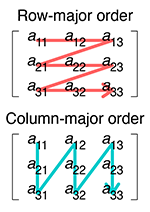
Row and column major order by Cmglee, CC BY-SA 4.0

The list of lists may have the rows separated in memory, they are written wherever there is space. The arrays in numpy are guaranteed to be contiguous. The data can be written across rows (row-major), or down the columns (col-major). To access a value, internally numpy's code looks something like this:

val = arr[i * i_stride + j * j_stride];

For row-major data, i_stride = 1 and j_stride = n_columns. For col-major data i_stride = n_rows and j_stride = 1. This can be extended into N dimensions by adding further strides.

NB In R you can use the built-in array type, with any vector of dimensions dim. The indexing is really intuitive and gives fast code. It's one of my favourite features of the language. Note there is also a matrix type, which uses exactly two dimensions and silently converts all entries to the same type -- use with care (particularly with apply, vapply is often safer).

Why are numpy arrays faster?

No type checking, as you're effectively using C code.
Less pointer chasing as memory is contiguous (see compiled languages).
Optimisations such as vectorised instructions are possible for the same reason.
Functions to work with the data have been optimised for you (particularly linear algebra). And in some cases preallocation of the memory is faster than dynamically sized lists (though in python this makes less of a difference as lists are pretty efficient).

Matrix multiplication

Simple matrix multiplication order in memory by Maxiantor, CC BY-SA 4.0

Let's compare summing values in a list of lists to summing a numpy array:

import numpy as np

def setup():
    xlen = 1000
    ylen = 1000

    rand_mat = np.random.rand(xlen, ylen)

    lol = list()
    for x in range(xlen):
        sublist = list()
        for y in range(ylen):
            sublist.append(rand_mat[x, y])
        lol.append(sublist)
    return rand_mat, lol

def sum_mat(mat):
    return np.sum(mat)

def sum_lol(lol):
    full_sum = 0
    for x in range(len(lol)):
        for y in range(len(lol[x])):
            full_sum += lol[x][y]
    return full_sum

def main():
    import timeit

    rand_mat, lol = setup()
    print(sum_mat(rand_mat))
    print(sum_lol(lol))

    setup_str = '''
import numpy as np
from __main__ import setup
from __main__ import sum_mat
from __main__ import sum_lol

rand_mat, lol = setup()
'''
    print(timeit.timeit("sum_mat(rand_mat)", setup=setup_str, number=100))
    print(timeit.timeit("sum_lol(lol)", setup=setup_str, number=100))

if __name__ == "__main__":
    main()

Which gives:

numpy sum: 500206.0241503447
list sum: 500206.0241503486

100x numpy sum time: 0.019256124971434474
100x list sum time: 9.559518916998059

A 500x speedup! Also note the results aren't identical, the implementations of sum cause slightly different rounding errors.

We can do a bit better using fsum:

def sum2_lol(lol):
    from math import fsum
    row_sum = [fsum(x) for x in lol]
    full_sum = fsum(row_sum)
    return full_sum

This takes about 2s (5x faster than the original, 100x slower than numpy) and gives a more precise result.

There are also advantages to preallocating memory space too, i.e. giving the size of the data first, then writing into the structure using appropriate indices. With the codon counting example, that might look like this:

def count_codons_numpy(seqs):
    # Precalculate codons and map them to integers
    bases = ['A', 'C', 'G', 'T']
    codon_map = dict()
    idx = 0
    for base1 in bases:
        for base2 in bases:
            for base3 in bases:
                codon = ''.join(base1 + base2 + base3)
                codon_map[codon] = idx
                idx += 1

    # Create a count matrix of zeros, and write counts directly into
    # the correct entry
    codon_len = int(len(seqs[0]) // 3)
    counts = np.zeros((codon_len, len(codon_map)), np.int32)
    for seq in seqs:
        for codon_idx in range(codon_len):
            codon = seq[codon_idx:(codon_idx + 3)]
            if not '-' in codon:
                counts[codon_idx, codon_map[codon]] += 1

    return counts

This is actually a bit slower than the above code as the codon_map means accesses move around in memory rather than being to adjacent locations (probably causing cache misses, but I haven't checked this.)

Sparse arrays

When you have numpy arrays with lots of zeros, as we do here, it can be advantageous to use a sparse array. The basic idea is that rather than storing all the zeros in memory, where we do have a non zero value (e.g. a codon count) we store the value, its row and column position in the matrix. As well as saving memory, some computations are much faster with sparse rather than dense arrays. They are frequently used in machine learning applications. For example see lasso regression which can use a sparse array as input, and jax for use in deep learning.

You can convert a dense array to a sparse array:

sparse_counts = scipy.sparse.csc_array(counts)
print(sparse_counts)

  (3, 0)        4889
  (4, 0)        4889
  (5, 0)        4889
  (6, 0)        4889
  (81, 0)       4889
  (82, 0)       613
  (94, 0)       3281
...

In python you can use scipy.sparse.coo_array to build a sparse array, then convert it into csr or csc form to use in computation.

In R you can use dgTMatrix, and convert to dgCMatrix for computation. The glmnet package works well with this.

Just-in-time compilation

We mentioned above one of the reasons python code is not as fast as the numpy equivalent is due to the type checking that is needed when it is run. One way around this is with 'just-in-time compilation', where python bytecode is compiled to (fast) machine code at runtime and before a function executes, and checking of types is done once when the function is first compiled.

One package that can do this fairly easily is numba. numba works well with simple numerical code like the sum above, but less well with string processing, data frames or other packages. It can even run some code on CUDA GPUs (I haven't tried it -- a quick look suggests it is somewhat fiddly but actually quite feature-complete).

In many cases, you can run numba by adding an @njit decorator to your function. NB I would always recommend using nopython=true or equivalently @njit as you otherwise you won't see when numba is failing to compile.

Exercise: Try running the sum_lol() and sum_lol2() functions using numba. Time them. Run them twice and time each run. Note that fsum won't work, but you can use sum. You will also want to use List from numba.

Expand the section below when you have tried this.

Sums with numba

import numpy as np
from numba import njit
from numba.typed import List

def setup():
    xlen = 1000
    ylen = 1000

    rand_mat = np.random.rand(xlen, ylen)

    lol = List()
    for x in range(xlen):
        sublist = List()
        for y in range(ylen):
            sublist.append(rand_mat[x, y])
        lol.append(sublist)
    return rand_mat, lol

@njit
def sum_mat(mat):
    return np.sum(mat)

@njit
def sum_lol(lol):
    full_sum = 0
    for x in range(len(lol)):
        for y in range(len(lol[x])):
            full_sum += lol[x][y]
    return full_sum

@njit
def sum2_lol(lol):
    row_sum = [sum(x) for x in lol]
    full_sum = sum(row_sum)
    return full_sum

def main():
    import timeit

    rand_mat, lol = setup()
    print(sum_mat(rand_mat))
    print(sum_lol(lol))

    setup_str = '''
import numpy as np
from __main__ import setup
from __main__ import sum_mat, sum_lol, sum2_lol

rand_mat, lol = setup()

# Compile the functions here
run1 = sum_mat(rand_mat)
run2 = sum_lol(lol)
run3 = sum2_lol(lol)
'''
    print(timeit.timeit("sum_mat(rand_mat)", setup=setup_str, number=100))
    print(timeit.timeit("sum_lol(lol)", setup=setup_str, number=100))
    print(timeit.timeit("sum2_lol(lol)", setup=setup_str, number=100))

if __name__ == "__main__":
    main()

This now gives the same result between both implementations:

500032.02596789633
500032.02596789633

and the numba variant using the built-in sum is a similar speed to numpy (time in s):

sum_mat 0.09395454201148823
sum_lol 2.7725684169563465
sum2_lol 0.08274500002153218

We can also try making our own array class with strides rather than using lists of lists:

@njit
def sum_row_ar(custom_array, x_size, x_stride, y_size, y_stride):
    sum = 0.0
    for x in range(x_size):
        for y in range(y_size):
            sum += custom_array[x * x_stride + y * y_stride]
    return sum

This about twice as fast as the list of list sum (1.4s), but still a lot slower than the built-in sums which can benefit from other optimisations.

Working with characters and strings

Needing arrays of characters (aka strings) is very common in sequence analysis, particularly with genomic data. It's very easy to work with strings in python (less so in R), but not always particularly fast. If you need to optimise string processing ultimately you may end up having to use a compiled language -- we will work through an example counting substrings (k-mers) from sequence reads in a later chapter.

That being said, numpy does have some support for working with strings by treating them as arrays of characters. Characters are usually coded as ASCII, which uses a single byte (8 bits: np.int8/u8/char/uint8_t depending on language).

Note that unicode, which is crucially needed for encoding emojis 🕴️ 🤯 🐈‍⬛ 🦉 and therefore essential to any modern research code, is a little more complex as it is variable length and uses an terminating character.

We can read our string directly into a numpy array of bytes as follows:

s = np.frombuffer(s.lower().encode(), dtype=np.int8)

Genome data often has upper and lowercase bases (a or A, c or C and so on) with no particular meaning assigned to this difference. It's useful to convert everything to a single case for consistency.

Here is an example converting the bases {a, c, g, t} into {0, 1, 2, 3}/{b00, b01, b10, b11} and using some bitshifts to do the codon counting:

@njit
def inc_count(codon_map, X):
    for idx, count in enumerate(codon_map):
        X[count, idx] += 1

def count_codons(seqs, n_codons):
    n_samples = 0
    X = np.zeros((65, n_codons), dtype=np.int32)
    for s in seqs:
        n_samples += 1
        s = np.frombuffer(s.lower().encode(), dtype=np.int8).copy()
        # Set ambiguous bases to a 'bin' index
        ambig = (s!=97) & (s!=99) & (s!=103) & (s!=116)
        if ambig.any():
            s[ambig] = 64
        # Shape into rows of codons
        codon_s = s.reshape(-1, 3).copy()
        # Convert to usual binary encoding
        codon_s[codon_s==97] = 0
        codon_s[codon_s==99] = 1
        codon_s[codon_s==103] = 2
        codon_s[codon_s==116] = 3
        # Bit shift converts these numbers to a codon index
        codon_s[:, 1] = np.left_shift(codon_s[:, 1], 2)
        codon_s[:, 2] = np.left_shift(codon_s[:, 2], 4)
        codon_map = np.fmin(np.sum(codon_s, 1), 64)
        # Count the codons in a loop
        inc_count(codon_map, X)

    # Cut off ambiguous
    X = X[0:64, :]

    return X, n_samples

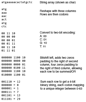Overview of algorithm Overview of the algorithm

This also checks for any non-acgt bases and puts them in an imaginary 65th codon, which acts as a bin for any unobserved data. Stops can also be removed. A numba loop is used to speed up the final count.

Overall this is about 50% faster than the dictonary implementation for this size of data, but is quite a bit more complex and likely error-prone. This type of processing can become worth it when the strings are larger, as we will see.

Alternative python implementations

We can also try alternative implementations of the python interpreter over the standard CPython. A popular one is pypy which can be around 10x faster for no extra effort. You can install via conda.

On my system for the sum benchmake, this ended up being 3-10x slower than CPython:

sum_lol 36.7518346660072
sum2_lol 56.79283958399901

but for the codon counting benchmark, was about twice as fast:

fn1: 2.63s
fn2: 0.83s

It costs almost nothing to try in many cases, but make sure you take some measurements.

Multithreading

Using multiple CPU cores is a very common optimisation strategy. Modern laptops have 4-10 cores, and HPC nodes usually have 32. These give the best case speedups, though often efficiency \(\frac{t_{\mathrm{serial}}}{t_{\mathrm{parallel}} \times N_{\mathrm{CPUs}}}\) is less than 100%.

Here we will use the terms threads, processes and CPUs interchangably, though note that in some settings they have important differences. (NB: Python has different executors for pools of threads and pools of processes -- see https://docs.python.org/3/library/concurrent.futures.html. In some cases one will achieve a speedup and the other won't! Typically, you should try using threads first.)

Some analysis does not require any use of shared memory or communication between threads. For example running the same program such as a genome assembler on 1000 different samples can be run as 1000 totally separate processes, and is probably best done as a job array or a pipeline like snakemake. These are known as 'embarrassingly parallel' tasks. You can also multithread embarrassingly parallel tasks when you are writing software, as it will be easier for many users to take advantage of.

What are good candidates for multithreading within a process? Usually where you have a part of your code that is particularly computationally intensive (usually as identified by some profiling) and uses the same variables/objects and therefore shared memory as the rest of the process.

When is it less likely to work? If multiple threads might write to the same variable or use the same resource then this makes things more complicated and often slower (but you can use atomic operations or mutexes to make this work). Additionally, making new threads usually has an overhead i.e. time cost, so the process being parallelised usually needs to run for a reasonable amount of time (at least greater than the cost of starting a new thread). Note, on Windows and OS X python uses spawn for each new thread, which starts a whole new python interpreter (potentially taking seconds). Unix uses fork which is faster. Bare in mind that if you are developing software you might need to support both methods!

A common structure in code that can be parallelised is a for loop where each iteration takes a non-negligible amount of time, as long as the loops do not depend on each other. Where the results need combining, a common approach is 'map-reduce' which applies a function to multiple data using map then applies a reduction function which combines the results from each of these processes.

Various options for multiprocessing are available in compiled languages and we will cover some of these later. Here we will use python's multiprocessing module to use multiple cores within one section of code.

Exercise Use a python multiprocessing Pool to parallelise the outer loop of the sum_lol() function from earlier. What is the speedup and efficiency? Plot this as the size of the list grows, and varying the size of the pool.

Compare with my attempt below when you are done:

Parallel sum

The setup is quite slow, so I will keep using numba even though it is excluded from the timing:

from numba import njit
import numpy as np
from multiprocessing import Pool
import time

@njit
def setup(N):
    xlen = N
    ylen = N

    rand_mat = np.random.rand(xlen, ylen)

    lol = list()
    for x in range(xlen):
        sublist = list()
        for y in range(ylen):
            sublist.append(rand_mat[x, y])
        lol.append(sublist)
    return lol

# Serial version
def sum_lol(lol):
    sum = 0
    for x in range(len(lol)):
        for y in range(len(lol[x])):
            sum += lol[x][y]
    return sum

# Parallel map which sums one sublist
def sum_list(sublist):
    partial_sum = 0
    for entry in sublist:
        partial_sum += entry
    return partial_sum

def run_test(N, threads):
    lol = setup(N)
    start_t = time.time_ns()

    if threads > 1:
        # map
        with Pool(processes=threads) as pool:
            partial_sums = pool.map(sum_list, lol)
        # reduce
        final_sum = sum_list(partial_sums)
    else:
        final_sum = sum_lol(lol)

    end_t = time.time_ns()
    time_ms = (end_t - start_t) / 1000000

    print(f"Time to sum {N**2} entries with {threads} threads: {time_ms}ms")

def main():
    for threads in range(1, 5):
        for N_exp in range(5):
            run_test(10**(N_exp), threads)

if __name__ == "__main__":
    main()

On OS X, this gives me the following:

Time to sum 1 entries with 1 threads: 0.004ms
Time to sum 100 entries with 1 threads: 0.009ms
Time to sum 10000 entries with 1 threads: 0.63ms
Time to sum 1000000 entries with 1 threads: 66.252ms
Time to sum 100000000 entries with 1 threads: 6856.647ms
Time to sum 1 entries with 2 threads: 369.239ms
Time to sum 100 entries with 2 threads: 350.236ms
Time to sum 10000 entries with 2 threads: 344.328ms
Time to sum 1000000 entries with 2 threads: 378.785ms
Time to sum 100000000 entries with 2 threads: 4554.182ms
Time to sum 1 entries with 3 threads: 372.856ms
Time to sum 100 entries with 3 threads: 360.495ms
Time to sum 10000 entries with 3 threads: 361.229ms
Time to sum 1000000 entries with 3 threads: 384.375ms
Time to sum 100000000 entries with 3 threads: 3399.802ms
Time to sum 1 entries with 4 threads: 394.478ms
Time to sum 100 entries with 4 threads: 375.59ms
Time to sum 10000 entries with 4 threads: 388.037ms
Time to sum 1000000 entries with 4 threads: 425.455ms
Time to sum 100000000 entries with 4 threads: 2956.621ms

For smaller lists, the time is always around 300-400ms on any multithreaded implementation, which is just the overhead of creating the Pool. For the larger list more threads is giving more speed, at around 75% efficiency for two threads, reducing to around 60% efficiency with four threads.

Here we are running a thread for each go around the outer loop, i.e. for x in range(len(lol)). We could also run threads to parallelise the inner loop too. What would be the advantages and disadvantages of this approach?

Returning results and shared memory

The above example is simple in that the function being parallelised takes a single iteraable and returns a single value (a scalar), so the return from Pool.map is a list of these scalars.

If you want to run a function which has other arguments, you can use partial to bind the other arguments before passing it as a closure to the map call.

If you want each thread to write results into (non-overlapping) parts of shared memory this is possible with SharedMemory introduced in python 3.8. This is also useful if you have very large arrays as input which would otherwise be copied across every thread increasing memory use.

We won't go into this much further, but here is an example of putting all of this together which assigns samples to a HDBSCAN model in parallel:

# Imports
from functools import partial
from tqdm.contrib.concurrent import thread_map, process_map
try:
    from multiprocessing import shared_memory
    from multiprocessing.managers import SharedMemoryManager
    NumpyShared = collections.namedtuple('NumpyShared', ('name', 'shape', 'dtype'))
except ImportError as e:
    sys.stderr.write("This code requires python v3.8 or higher\n")
    sys.exit(0)

def assign_samples(chunk, X, y, model, n_samples, chunk_size):
    # Load in shared memory
    if isinstance(X, NumpyShared):
        X_shm = shared_memory.SharedMemory(name = X.name)
        X = np.ndarray(X.shape, dtype = X.dtype, buffer = X_shm.buf)
    if isinstance(y, NumpyShared):
        y_shm = shared_memory.SharedMemory(name = y.name)
        y = np.ndarray(y.shape, dtype = y.dtype, buffer = y_shm.buf)

    # Set range thread is operating on
    start = chunk * chunk_size
    end = min((chunk + 1) * chunk_size, n_samples)

    # Run the prediction for this range
    y[start:end] = hdbscan.approximate_predict(model.hdb, X[start:end, :])[0]

# Set output to zeros
y = np.zeros(n_samples, dtype=int)
block_size = 100000
with SharedMemoryManager() as smm:
    # Make a shared memory array for input X and copy data into it
    shm_X = smm.SharedMemory(size = X.nbytes)
    X_shared_array = np.ndarray(X.shape, dtype = X.dtype, buffer = shm_X.buf)
    X_shared_array[:] = X[:]
    X_shared = NumpyShared(name = shm_X.name, shape = X.shape, dtype = X.dtype)

    # Make a share memory array for output y and copy data into it
    shm_y = smm.SharedMemory(size = y.nbytes)
    y_shared_array = np.ndarray(y.shape, dtype = y.dtype, buffer = shm_y.buf)
    y_shared_array[:] = y[:]
    y_shared = NumpyShared(name = shm_y.name, shape = y.shape, dtype = y.dtype)

    # Run the function `assign_sample` multithreaded
    thread_map(partial(assign_samples,
                                X = X_shared,
                                y = y_shared,
                                model = dbscan_model,
                                n_samples = n_samples,
                                chunk_size = block_size),
                        range((n_samples - 1) // block_size + 1),
                        max_workers=threads)

    # Copy results back into y
    y[:] = y_shared_array[:]

return y

Notes:

thread_map from tqdm is used, to provide a progress bar.
partial is used to bind the arguments of assign_samples, as the map only iterates over the first argument.
A SharedMemoryManager is used to share numpy arrays between threads without copying them.
The main code needs to set these arrays up using a buffer.
The called function needs to unpack them.
Non-overlapping rows of the array each thread operates on are manually calculated.

Memory optimisation

It's often the case that you want to reduce memory use rather than increase speed. Similar tools can be used for memory profiling, however in python this is more difficult. If memory is an issue, using a compiled language where you have much more control over allocation and deallocation, moving and copying usually makes sense.

In python, using preallocated arrays can help you control and predict memory, and ensuring you don't copy large objects or delete them after use is also a good start.

Some other tips:

Avoid reading everything into memory and compute 'on the fly'. The above code reads in all of the sequences first, then processes them one at a time. These could be combined, so codons counts are updated after each sequence is read in, so then only one sequence needs to fit in memory.
You can use disk (i.e. files) to move objects in and out of memory, at the cost of time.
Memory mapping large files you wish to modify part of can be an effective approach.

Writing extensions in compiled code

It is possible to write C/C++ code and call it from python using Cython. Instead, I would highly recommend either the pybind11 or nanobind packages which make this a lot easier.

The tricky part is writing your setup.py and Makefile/CMakeLists.txt to get everything to work together. If you are interested in this approach, examples from some of our group's packages may be helpful:

sketchlib calls C++ and CUDA code from python.
mandrake does the same, but also returns an object used in the python code.
ggcaller uses both python and C++ code throughout.

Please feel free to adapt and reuse the build approach taken in any of these.

Other optimisations

For data science, have a look at the following packages for tabular data:

cuDF - GPU accelerated data frames: https://docs.rapids.ai/api/cudf/stable/
Apache arrow and Parquet format: https://arrow.apache.org/docs/python/index.html

Notes (for next year)

Code should probably be given, rather than written
This isn't doable for R users
1st part unclear what should be read/checked
Which reading frames
Snakeviz a good tool for visualisation of profiles
Better examples of fasta and expected output
Bitshift example is the wrong way round

Intermediate Research Programming Course